---

Introduction on coordination games

Coordination games describe situations that reward conformity. Individuals gain high payoffs if they all choose the same strategy and lower payoffs if some individuals deviate. Subclasses of coordination games exist for the many possible payoff structures that specify the different rewards of achieving coordination on the various strategies, the punishment that deviators receive, and how conformists are hurt by the deviators.

The most stringent type of coordination game is called pure coordination game in which players receive payoff a>0 if they all play Strategy 1, b>0 if they all play Strategy 2, and 0 otherwise. If a>b, we may imagine this as a model of adopting a new technology: players gain the most by agreeing to use the more efficient Strategy 1 and gain lower payoffs by sticking with the less efficient Strategy 2. However, if coordination fails, chaos ensues, leaving everyone with zero payoffs (Table 1).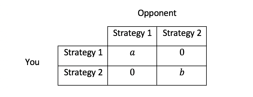

Table 1: Payoffs of a pure coordination game with two players and two strategies

Once coordination is achieved, the winning strategy is fixated while the losing strategy goes extinct. The game is, in appearance, over, and unless one knows to look for them, the losing strategies cannot be observed, so these games can be hard to identify in applications.

An evolutionary game of cancer cells with two strategies (types) is characterized by four payoff values. Let \(r_i\) and \(d_i\), for \(i=1,2\), denote the payoff/fitness of a type i cell in its own environment, and in the other type’s environment, respectively. The full game is shown in Table 3. We can assume that \(r_1≥r_2\) without loss of generality (Table 2).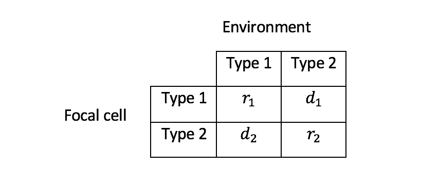

Table 3: A game between two cancer cell types

For this to be a coordination game, the payoffs need to satisfy \(r_1>d_1, r_2>d_2\) and if \(r_2>d_1\). See our Supplementary Information for the detailed conditions of coordination games.

Two candidates for coordination games in cancer

“Driver genes” may help identify coordination games. In many cancers, a specific gene mutation is observed in almost all cells and is vital for the proliferation of cancer cells. Perhaps the best example is the oncogenic mutation of Epidermal Growth Factor in lung cancers (accounting for 15-20% of lung cancers). Unlike most lung cancer cohorts in which prolonged smoking and exposure to air pollutants are clear risk factors, EGFR-mut cancers tend to occur in younger patients who are non-smokers. For these patients, the EGFR-mutation occurs in essentially all the cancer cells of the primary and metastatic tumors. Furthermore, the mutational burden in EGFR-mut lung cancer is significantly smaller than EGFR WT lung cancers, indicating a molecularly more homogeneous intra-tumoral population. We propose that EGFR-mut versus EGFR WT lung cancers represent a coordination game.

Treatment of EGFR-mut lung cancers with tyrosine kinase inhibitors (TKI) that specifically target the EGFR-mut function results in a complete or partial response in most (75%) patients. However, response is temporary and the cancer progresses within 12 to 14 months. At least 7 different strategies permit the lung cancer cells to overcome the TKIs (mechanisms in 15% of cases are still unknown). It has been noted that in many cases, resistance takes the form of the cancer cells losing the EGFR-mut and becoming EGFR-WT lung cancers. As a coordination game, treating the EGFR-mut may simply shift the cancer to an alternate stable state.

Another subset of lung cancers (about 40%) have an oncogenic KRAS mutations indicating that driver mutations are, to some extent, substitutable. But cancer cells with different driver mutations may not be able to coexist within the same patient or tumor. In the case of non-small-cell lung cancer, for example, the driver mutations in KRAS and EGFR seem to be mutually exclusive, suggesting that, once a cancer population has one, the other is selected against. Thus, one or the other is beneficial, but both are harmful to the cancer cell, a necessary condition of a coordination game.

Our second candidate is breast cancer. In patients with breast cancer, the commonly expressed beta-arrestin isoforms β-arrestin 1; ARRB2, and β-arrestin 2; ARRB3 may form the biological basis for a coordination game. β-arrestins function as “terminators” of G protein-coupled receptor (GPCR) signaling. More recently, β-arrestins, through their scaffolding functionality, have also been shown to serve as signal “transducers”.

Studies have reported a change in the expression of β-arrestins in breast cancer cells and patient tumors, where changes in their expression correlate with poor patient survival, with β-arrestin 2 expression serving as a prognostic biomarker in breast cancer. Investigations of several human genomic datasets revealed that β-arrestin 1 is downregulated in triple negative breast cancer, the most aggressive breast cancer. This suggests that cancer cell fitness is maximized by changing the expression of one but not both β-arrestins. Changing one promotes self-sufficiency in proliferative signaling, while keeping the other unchanged maintains the necessary cellular functions.

While these observations can explain how a co-adapted set of genes coordinates cellular processes within a cancer cell, it does not necessarily qualify as a coordination game for explaining why all cells of the patient's cancer show one pattern of changes in β-arrestin and not the other. The coordination game may result from the way β-arrestins control aspects of cell-cell signaling through the regulation of GPCR activity, as well as other cell surface receptors. In this case, the value of a particular isoform of β-arrestin for successful cell-cell communication within the tumor may be determined by the unified expression of this isoform by surrounding cancer cells. That is, the dominant β-arrestin isoform may define rules of the road for all cancer cells.

Cancer growth driven by a coordination game

Our model resembles a Lotka-Volterra competition model with two phenotypes. Our main addition is the coordination game in Table 3 as the “engine” of tumor growth. The components are summarized in Table 4.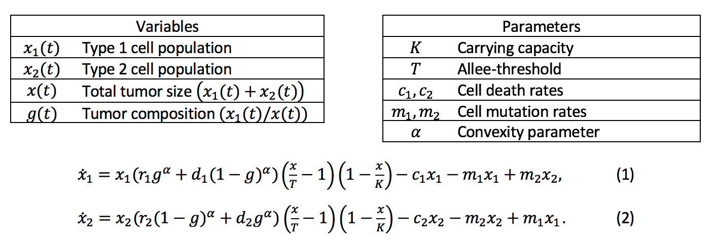

Table 4: A model of cancer growth governed by a coordination game

Most of the model’s components behave identically to Lotka-Volterra competition models: the environment has a carrying capacity K and an extinction threshold T that are shared by the two populations. The populations have type-specific death rates, \(c_1,c_2\) as well as type-specific mutation rates \(m_1,m_2\), by which the two types mutate into one another, capturing the phenotypic variability and instability of cancer.

The type’s growth rates are governed by the coordination game. Purely type 1 and type 2 tumors grow at rates \(r_1\) and \(r_2\), respectively. The types’ growth rates in a mixed tumor are given by a combination of their fitness in the own environment, \(r_i\), and their fitness in the opposing type’s environment, \(d_i\). The convexity parameter \(\alpha≥1\) determines the growth rates’ frequency-dependence (see our Supplementary Information for a detailed discussion).

We illustrate this model in Figure 1. The maximum size of the tumor (the upper bound of the region with positive total cell growth) is V-shaped: more homogeneous tumors can sustain higher populations. The extinction zone (the lower bound) is its flipped mirror image: more homogeneous tumors are easier to sustain. The heatmaps of tumor growth (Figure 1) reveal two “peaks” of tumor fitness at the two ends of the composition, divided by a low fitness “valley” in between.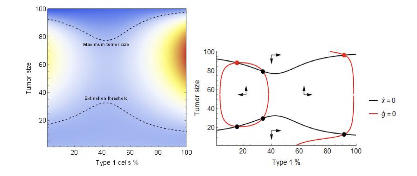

Figure 1: The heat map and phase diagram of tumor fitness and composition. Parameters: \(r_1=0.25,r_2=0.17, d_1=d_2=0,K=100,T=10,c_2=0.1,c_1=0.05\).

The phase diagram reveals the deeper mechanics. At the extreme levels of tumor composition, mutation pushes the system “inward” to a more heterogeneous tumor. However, in the interior, the coordination game pushes the tumor “outward”, to a more homogeneous tumor, creating two stable equilibria where composition is mostly but not completely homogeneous.

Therapy and coordination games

Here we discuss cytotoxic therapy, which increases the cells’ death rates. In our paper we propose and simulate a second type of therapy which affects the cell types’ mutation rates.

Increasing the death rate is a direct attack on the tumor, typically with the goal of driving the cancer cell population to extinction. These direct attacks on the tumor’s size, however, are not always enough as the tumor evolves resistance, rendering the cytotoxic agent ineffective. However, if the different types react differently to the cytotoxic agent, e.g. the two types represent therapy sensitivity and resistance, a treatment can be designed to push the tumor to the heterogeneous, low-fitness region and collapse the cancer population.

To illustrate this, consider the model defined by (3)-(4). To fully showcase the strength of the coordination game we consider the model without an extinction threshold. The discrete variables \(\gamma_1 (t),\gamma_2 (t)\) correspond to cytotoxic therapy; \(\gamma_i (t)=\gamma_i\) for some \(\gamma_i≥0\) in time instances when the patient undergoes treatment, and \(\gamma_i (t)=0\) otherwise.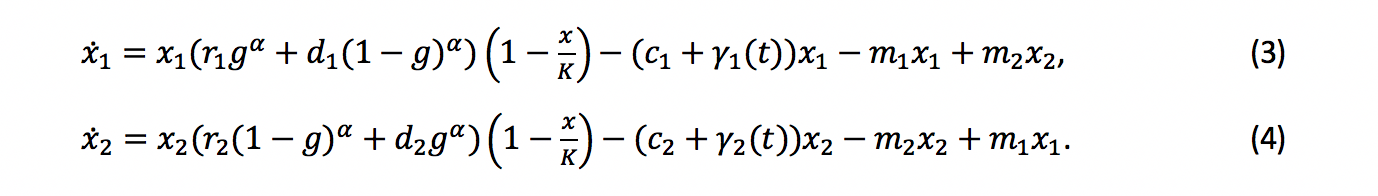

We consider a classic sensitive-resistant model: type 1 is sensitive and thus therapy raises its death rate by a value γ_1>0, while type 2 is resistant, so its death rate is unaffected, amounting to \(\gamma_2=0\). While any difference between the types’ reaction to the cytotoxic agent can be leveraged, our setting captures an extreme case for convenience of illustration.

Figure 3 illustrates the system given by (3)-(4) with therapy off (left panel), and therapy on (right panel). Without therapy, the system is reminiscent of the top half of Figure 2’s right panel, producing two stable equilibria. The near-vertical composition zero-isocline at g=40% marks the border between the basins of attraction: small tumors with more than 40% type 1 cells will grow to coordinate on the type 1 equilibrium, those with less than that will grow to coordinate on the type 2 one. As type 2 is resistant, continuous therapy leads to a single stable equilibrium dominated by type 2 cells.

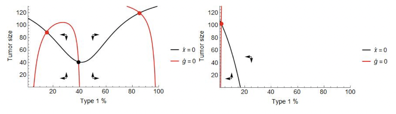
Figure 3: The phase diagram of the model defined by (3)-(4) with cytotoxic therapy off (left) and on (right). Parameters: \(r_1=0.4,r_2=0.2,d_1=d_2=0,K=150,c_1=c_2=0.05,m_1=m_2=0.01,γ_1=0.4\).

Imagine that, at the initiation of the therapy, the patient presents with a sensitive tumor. Without intervention the patient progresses when his or her tumor burden reaches a critical mass of sensitive cells. Under continuous cytotoxic therapy, after a good initial response in tumor size, the population begins climbing again once it achieves coordination on the resistant type and the patient progresses (Figure 4, top left panel). However, in doing so, the system transits through the unstable middle region where the tumor is heterogeneous, and its fitness – sans therapy – is small. Stopping therapy at that point traps the tumor in the fitness valley. As this region is unstable, the tumor will spend some time here, then reach coordination on one type or the other. Whether it achieves coordination on the sensitive type or the resistant one depends on whether the tumor reached the resistant basin of attraction. If therapy is stopped at a point when composition is below the threshold 40%, the tumor will coordinate on the resistant type (Figure 4, top right). If, however, treatment is stopped earlier, the sensitive population will rebound and coordination is achieved on type 1 instead (Figure 4, bottom left). In both cases the patient’s progression time rises as the tumor spends time in the low fitness region. If the resistant type ends up dominating, control over the tumor is lost. On the other hand, if sensitive cells rebound, the process may be repeated, possibly trapping the tumor on multiple occasions and buying the patient more time, until control is finally lost (Figure 4, bottom right). The key difference between coordination games and other models of resistance and adaptive therapies in the discontinuity between the two attractors.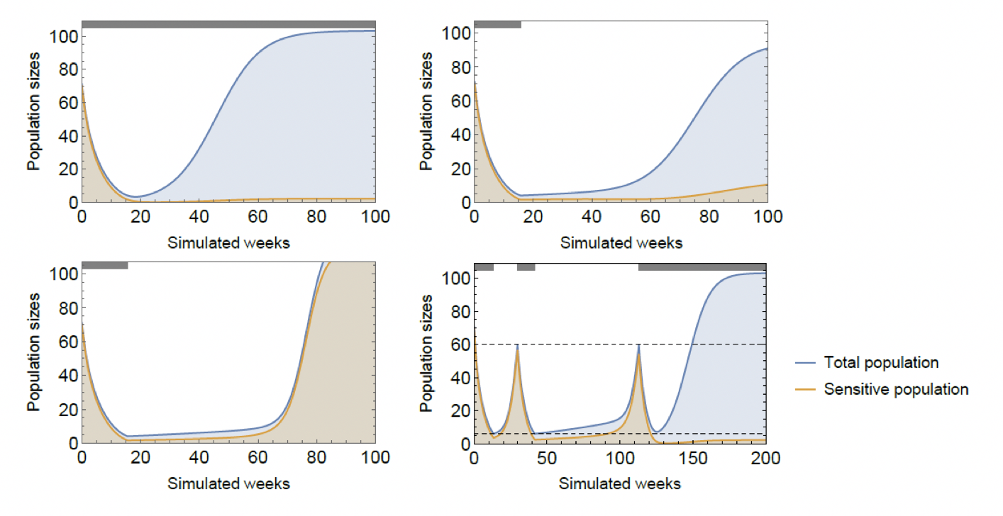

Figure 4: The effects of continuous cytotoxic therapy (top left), stopping at g=39% (top right), stopping at g=40% (bottom left), and an on-off treatment strategy (bottom right). Parameters: \(r_1=0.4,r_2=0.2,d_1=d_2=0,K=150,c_1=c_2=0.05,m_1=m_2=0.01,γ_1=0.4\).

A good application of such an on-off therapy can put both the tumor’s size and composition in a recurring, persistent cycle, and thus can stave off tumor progression indefinitely (Figure 5, left panel). Moreover, under ideal circumstances, the cycles in composition can be sustained as the tumor’s size declines, and the tumor can be driven extinct (Figure 5, right panel). ‘Ideal circumstances’ here refers to the fact that extinction through therapy requires for the physician to monitor the tumor’s composition, which is not within reach. Cycles require monitoring of the tumor’s size and are thus, practicable.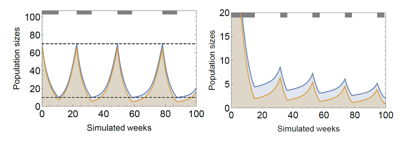

Figure 5: Successful adaptive therapy (left) and extinction therapy (right). The shown adaptive strategy is to apply therapy until cancer population falls to 10, then stop therapy and restart when it reaches 70. Under the extinction strategy, therapy is applied until tumor composition falls below 45% and restarted when it reaches 75%. Parameters: \(r_1=0.4,r_2=0.2,d_1=d_2=0,K=150,c_1=c_2=0.05,m_1=m_2=0.01,γ_1=0.4\).

We note that while other models of adaptive therapies exist, there are no eco-evolutionary models to our knowledge that capture the persistent cycles shown to exist in mouse trials with a basis in cell-to-cell interactions. In other models, sensitivity is not an evolutionary stable “enough” for the tumor for the cycles to truly recur.

We invite readers to check out our preprint and our supplementary information document. Comments and thoughts are very welcome!

Link to paper.
Link to supplementary information.