---

Disclaimer: Running the code requires Python 3 with PyTorch 2+ to be installed and a Bash-compatible shell. NVIDIA GPU is recommended for faster training, but it is not necessary.

What are genomic copy numbers?

Cancer is characterized by the uncontrolled growth of cells, typically caused by disruption in their normal cell function. Typically, these disruptions often result from DNA mutations. Some of these mutations are small - single nucleotide variations or substitutions, but most cancers also exhibit large-scale alterations in the DNA that produce a widely varying number of gene copies within cells.

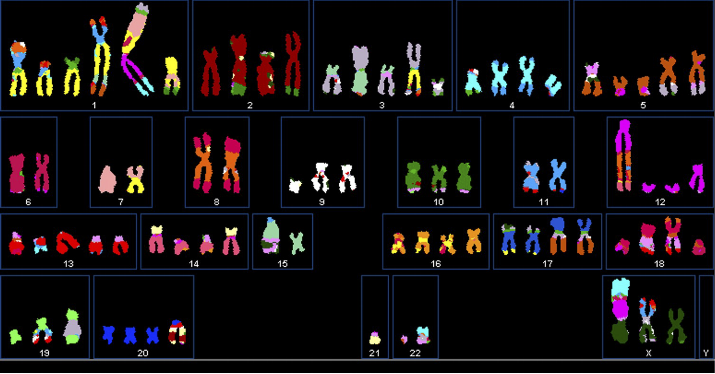
These large-scale genomic structural changes lead to loss of genes that prevent cancer from forming (tumor suppressors), while amplifying copies of genes that promote cell growth (oncogenes). By sequencing the DNA of these cells, we can identify these changes, which happen quite often in cancer-type specific regions.

The sequenced DNA is generally in the form of FASTA files that are then aligned to a reference genome (e.g. hg38), and finally, copy numbers values for each of the two alleles are derived using copy number callers. The output generally includes the following:

• Chromosome
• Start and End position of the genomic segment
• Copy Number (either total or allele-specific)

What is CNSistent?

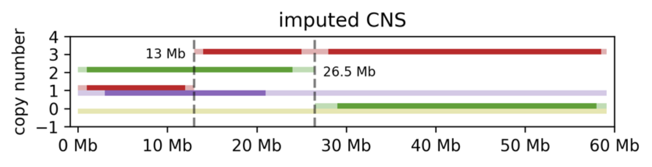
One of the advantages of working with copy number profiles is that they are not biometric and therefore can be published without the need for access restrictions. This allows us to accumulate data over time from multiple studies to build datasets of sufficient size. However, the data obtained from different studies is not always directly comparable, because of different technologies, and/or use of different resolutions or pre-processing methods. This can lead to missing values in certain genomic segments, reduced sample quality and most commonly, produce inconsistent segment lengths across different copy number profiles. CNSistent aims to address this issue by joint processing and filtering the copy number profiles. CNSistent can:

1. Imputation: derive missing values from the neighboring segments to create a continuous profile
2. Filter samples: remove samples with low quality data or low mutational activity (for example in virus-mediated cancers)
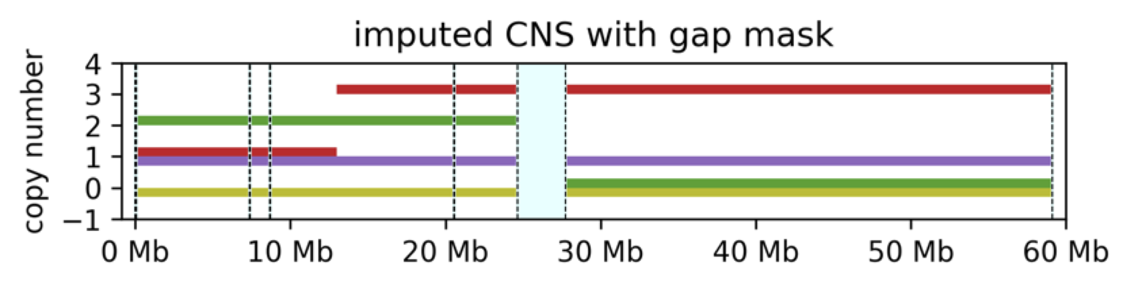
3. Filter regions: remove regions with low mappability or high variability
4. Consistent segmentation: create segments with aligned boundaries across samples for meaningful comparison.

Below is a sample CNSistent data-processing pipeline:

We can also see that s2 had no copy number values for CN2. This is sometimes the case with real data; however, such a massive loss considerably decreases reliability of the data. To address this, CNSistent also allows to filter out data with too many missing values or low chromosomal instability (see our publication for details).

Cancer classification from Copy Number Segments using CNSistent and PyTorch

Now that we know how to obtain good quality copy numbers, we will now show you how to make a classifier based on a Convolutional Deep Neural Network that distinguishes lung cancer subtypes. In particular, we will distinguish Adenocarcinoma from Squamous cell carcinoma, using their genomic copy number profiles.

Processing cancer samples using CNSistent

First, we will clone the repository and the data and set it to the version used in this text:

git clone git@bitbucket.org:schwarzlab/cnsistent.git
cd cnsistent
git checkout MO

Since the data we will be using is inside the repository (~1GB of data), it can take a few minutes to download.

Inside the repository is a requirements.txt file that lists all the dependencies that can be installed using pip install -r requirements.txt (creating a virtual environment first is recommended).

Once the requirements are installed, CNSistent can be installed by running pip install -e . in the same folder. The -e flag installs the package from its source directory, which is necessary for access to the data through the API.

The repository contains raw data from three datasets: TCGA, PCAWG, and TRACERx. This needs to be pre-processed first. This can be done by running the following script:

bash ./scripts/data_process.sh

Now, we have processed datasets and can load them using the CNSistent data utility library:

import cns.data_utils as cdu
samples_df, cns_df = cdu.main_load("imp") # "imp" stands for imputed data
print(cns_df.head())

sample_id	chrom	start	end	major_cn	minor_cn
SP101724	chr1	0	27256755	2	2
SP101724	chr1	27256755	28028200	3	2
SP101724	chr1	28028200	32976095	2	2
SP101724	chr1	32976095	33354394	5	2
SP101724	chr1	33354394	33554783	3	2
...	...	...	...	...	...

This table shows the copy number data with the following columns:

• sample_id - the identifier of the sample
• chrom - chromosome number
• start - the start position of the segment (0-indexed inclusive)
• end - the end position of the segment (0-indexed exclusive)
• major_cn - the number of copies of the major allele (the bigger of the two)
• minor_cn - the number of copies of the minor allele (the smaller of the two)

In the first row of the table given above, we can therefore see a segment stating that sample SP101724 has 2 copies of the major allele and 2 copies of the minor allele (4 in total) in the region of chromosome 1 from 0 to 27.26 megabase.

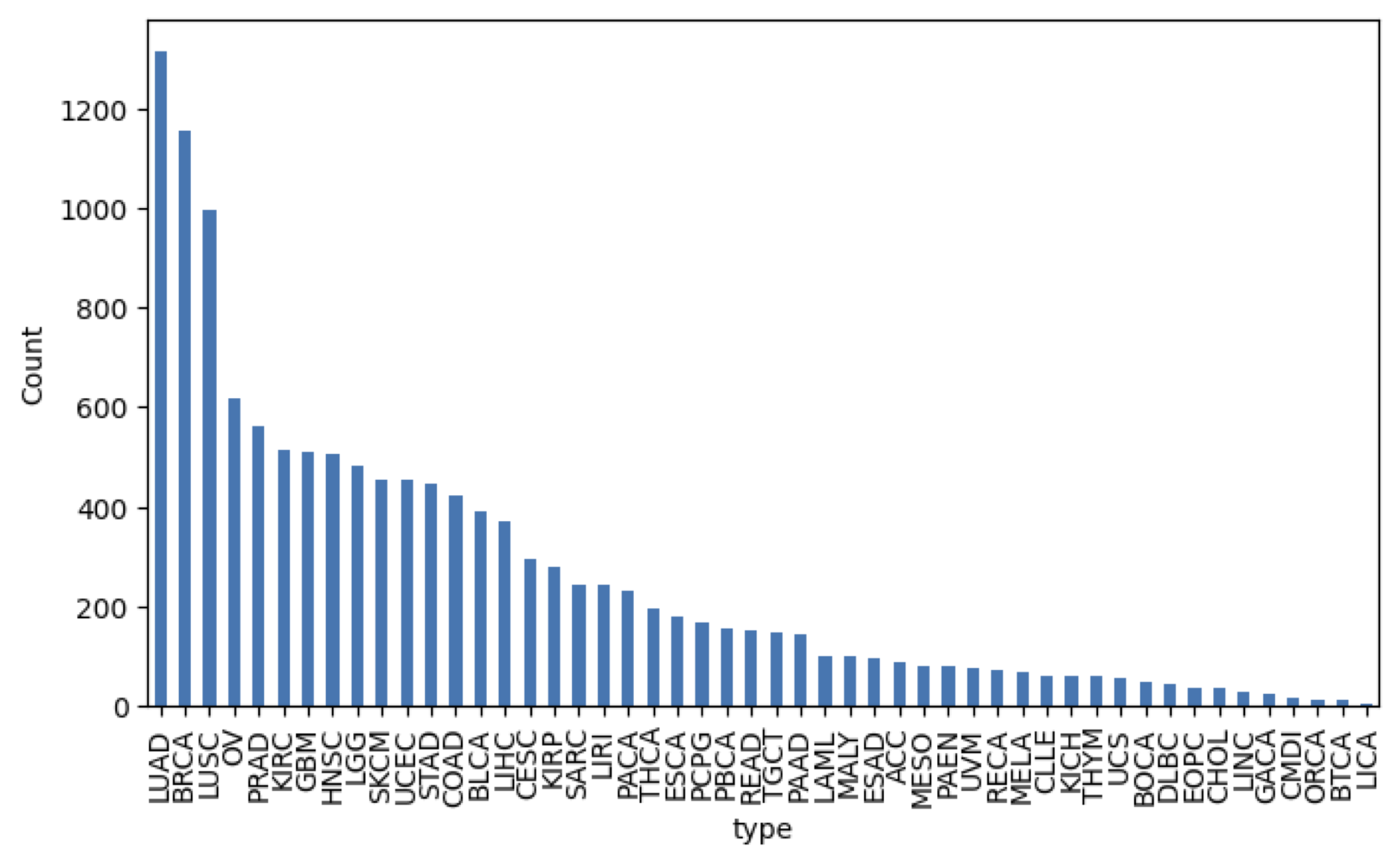
The second dataframe we loaded, samples_df, contains the metadata for the samples. For our tutorial, only the type is relevant. We can investigate the available types by running:

import matplotlib.pyplot as plt
type_counts = samples_df["type"].value_counts()
plt.figure(figsize=(10, 6))
type_counts.plot(kind='bar')
plt.ylabel('Count')
plt.xticks(rotation=90)	

Segmentation

In the example shown above, we observe a potential problem with the data - the lengths of the individual segments are not uniform. The first segment is 27.26 megabase long, while the second one is only 0.77 megabase long. This is a problem for the neural network, which expects the input to be of a fixed size.

We could technically take all existing breakpoints and create segments between all breakpoints in the dataset, also called minimum consistent segmentation. This would however result in a huge number of segments - a quick check using len(cns_df["end"].unique()) shows that there are 823652 unique segments.

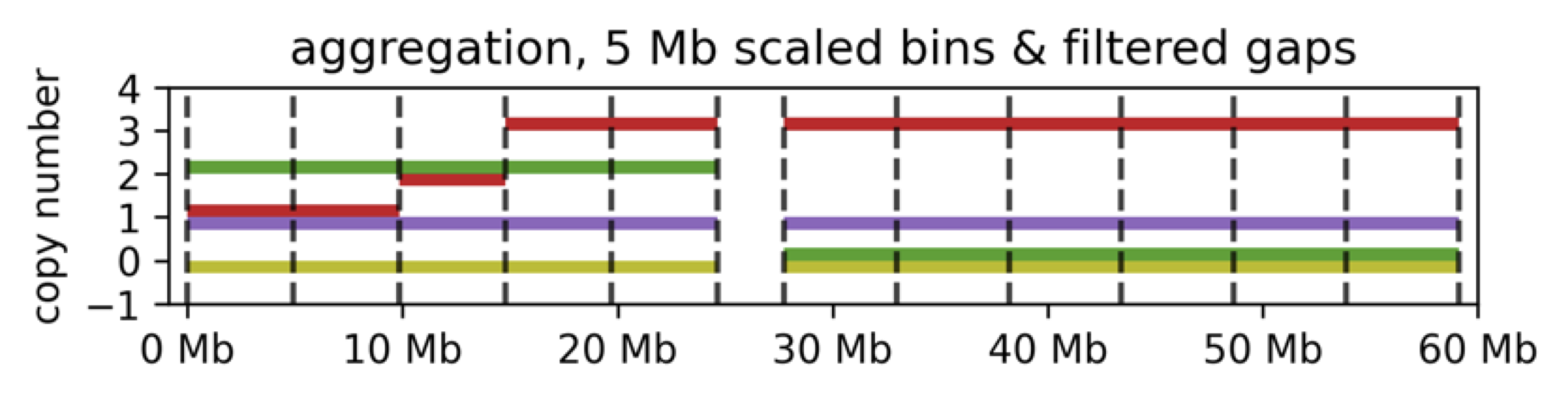
Alternatively, we can use CNSistent to create a new segmentation using a binning algorithm. This will create segments of a fixed size, which can be used as input to the neural network. In our work we determined that 1-3 megabase segments provide the best trade-off between accuracy and overfitting. We first create the segmentation and then apply it to obtain new CNS files using the following Bash script:

threads=8
cns segment whole --out "./out/segs_3MB.bed" --split 3000000 --remove gaps --filter 300000  
for dataset in TRACERx PCAWG TCGA_hg19; 
do
	cns aggregate ./out/${dataset}_cns_imp.tsv --segments ./out/segs_3MB.bed --out ./out/${dataset}_bin_3MB.tsv --samples ./out/${dataset}_samples.tsv --threads $threads
done

The loop processes each dataset separately, while maintaining the same segmentation. The --threads flag is used to speed up the process by running the aggregation in parallel, adjusting the value according to the number of cores available.

The --remove gaps --filter 300000 arguments will remove regions of low mappability (aka gaps) and filter out segments shorter than 300 kilobases. The --split 3000000 argument will create segments of 3 megabases.

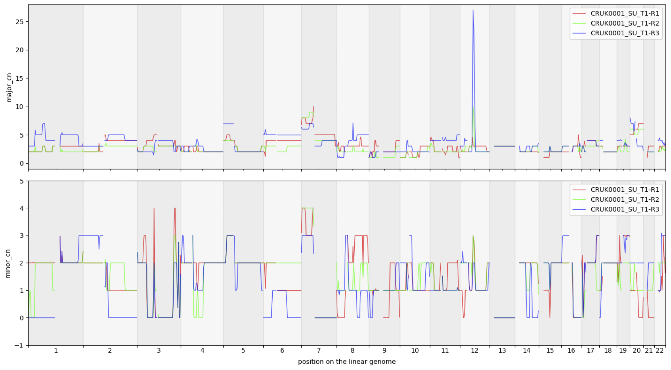
Once the data has been segmented, the new segments can be loaded. We use the "3MB" name specified above to load the segments with a utility function. Since we are classifying between two types of cancer, we can filter the samples to only include the relevant types, "LUAD" (adenocarcinoma) and "LUSC" (squamous cell carcinoma) as shown in the sample:

import cns
samples_df = samples_df.query("type in ['LUAD', 'LUSC']")
_, cns_df = cdu.main_load("3MB")
cns_df = cns.select_CNS_samples(cns_df, samples_df)
cns_df = cns.only_aut(cns_df)
cns.fig_lines(cns.cns_head(cns_df, n=3))	

The neural network model

First we define a deep convolutional neural network with three layers:

import torch.nn as nn

class CNSConvNet(nn.Module):
	def __init__(self, num_classes):
		super(CNSConvNet, self).__init__()
		self.conv_layers = nn.Sequential(
			nn.Conv1d(in_channels=2, out_channels=16, kernel_size=3, padding=1),
			nn.ReLU(),
			nn.MaxPool1d(kernel_size=2),
			nn.Conv1d(in_channels=16, out_channels=32, kernel_size=3, padding=1),
			nn.ReLU(),
			nn.MaxPool1d(kernel_size=2),
			nn.Conv1d(in_channels=32, out_channels=64, kernel_size=3, padding=1),
			nn.ReLU(),
			nn.MaxPool1d(kernel_size=2)
		)
		
		self.fc_layers = nn.Sequential(
			nn.LazyLinear(128),
			nn.ReLU(),
			nn.Dropout(0.5),
			nn.Linear(128, num_classes)
		)
		
	def forward(self, x):
		x = self.conv_layers(x)
		x = x.view(x.size(0), -1) 
		x = self.fc_layers(x)
		return x

This is a bottleneck deep CNN with 2 input channels - one for each allele - and 3 convolutional layers using 1D kernels of size 3 and ReLU activation function. The convolutional layers are followed by max pooling layers with kernel size of 2. Convolution is traditionally used for edge detection, which is useful for us as we are interested in changes in the copy number, i.e. the edges of the segments.

The output of the convolutional layers is flattened and passed through two fully-connected layers with dropout. The LazyLinear layer connects the output of 64 stacked channels into one layer of features without us needing to calculate how many nodes there are at the end of the convolution. This is where most of our parameters are, therefore we also apply dropout to prevent overfitting.

Training the model

First we have to convert from dataframes to Torch tensors. We use a utility function bins_to_features, which creates a 3D feature array of the format (samples, alleles, segments). In the process we also split the data into training and testing sets in the 4:1 ratio:

import torch
from torch.utils.data import TensorDataset, DataLoader
from sklearn.preprocessing import LabelEncoder
from sklearn.model_selection import train_test_split

# convert data to features and labels
features, samples_list, columns_df = cns.bins_to_features(cns_df)

# convert data to Torch tensors
X = torch.FloatTensor(features)
label_encoder = LabelEncoder()
y = torch.LongTensor(label_encoder.fit_transform(samples_df.loc[samples_list]["type"]))  

# Test/train split
X_train, X_test, y_train, y_test = train_test_split(X, y, test_size=0.2, random_state=0)

# Create dataloaders
train_loader = DataLoader(TensorDataset(X_train, y_train), batch_size=32, shuffle=True)
test_loader = DataLoader(TensorDataset(X_test, y_test), batch_size=32, shuffle=False)	

We can now train the model using the following training loop with 20 epochs. The Adam optimizer and CrossEntropy loss are typically used for classification tasks, we therefore use them here as well:

from torch import optim

# setup the model, loss, and optimizer
device = torch.device('cuda' if torch.cuda.is_available() else 'cpu')
model = CNSConvNet(num_classes=len(label_encoder.classes_)).to(device)
criterion = nn.CrossEntropyLoss()
optimizer = optim.Adam(model.parameters(), lr=0.001)

# Training loop
num_epochs = 20
for epoch in range(num_epochs):
	model.train()
	running_loss = 0.0
	
	for inputs, labels in train_loader:
		inputs, labels = inputs.to(device), labels.to(device)
		
		# Clear gradients
		optimizer.zero_grad()
		
		# Forward pass
		outputs = model(inputs)
		loss = criterion(outputs, labels)
		
		# Backward pass and optimize
		loss.backward()
		optimizer.step()
		
		running_loss += loss.item()
	
	# Print statistics
	print(f'Epoch {epoch+1}/{num_epochs}, Loss: {running_loss/len(train_loader):.4f}')

After the training we can evaluate the model and print the confusion matrix:

import numpy as np
from sklearn.metrics import confusion_matrix
import seaborn as sns

# Loop over batches in the test set and collect predictions
model.eval()
y_true = []
y_pred = []
with torch.no_grad():
	for inputs, labels in test_loader:
		inputs, labels = inputs.to(device), labels.to(device)
		outputs = model(inputs)
		y_true.extend(labels.cpu().numpy())
		y_pred.extend(outputs.argmax(dim=1).cpu().numpy())
		_, predicted = torch.max(outputs.data, 1)

# Calculate accuracy and confusion matrix
accuracy = (np.array(y_true) == np.array(y_pred)).mean()
cm = confusion_matrix(y_true, y_pred)

# Plot the confusion matrix
plt.figure(figsize=(3, 3), dpi=200)
sns.heatmap(cm, annot=True, fmt='d', cmap='Blues', xticklabels=label_encoder.classes_, yticklabels=label_encoder.classes_)
plt.xlabel('Predicted')
plt.ylabel('True')
plt.title('Confusion Matrix, accuracy={:.2f}'.format(accuracy))
plt.savefig("confusion_matrix.png", bbox_inches='tight')

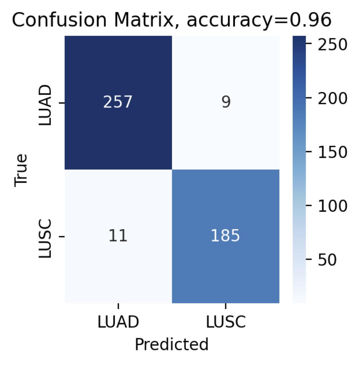
And voila! The confusion matrix shows that our model can distinguish between adenocarcinoma and squamous cell carcinoma with 96% accuracy. Note that your results may slightly vary based on the type of GPU/CPU, version of CUDA, or NVIDIA drivers.

Conclusion

This has been a quick introduction to copy-number data processing, segmentation, and classification using CNSistent and PyTorch. There are, of course, many additional considerations to be made, e.g. how to treat the multi-region data to avoid leakage between training and test sets. For details, please refer to our pre-print CNSistent integration and feature extraction from somatic copy number profiles.

CNSistent has been developed as work of the Institute for Computational Cancer Biology at the University Hospital Cologne, Germany.