---

Despite major strides in the treatment of cancer, the development of drug resistance remains a major hurdle. One strategy which has been proposed to address this is the sequential application of drug therapies where resistance to one drug induces sensitivity to another drug, a concept called collateral sensitivity. (Figure 1A) Particularly, there is utility in a drug sequence which completes a cycle of such relationships ¹ (e.g., the three drugs connected by the red arrows in Figure 1B). With such cycles, one could, in theory, generate infinitely long drug sequences which can be used in long term therapy to mitigate the evolution of resistance in a tumor. In light of this, we developed a mathematical model and found the optimal therapeutic strategy based on the model. ^2,3

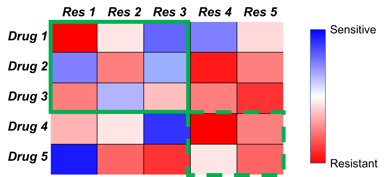
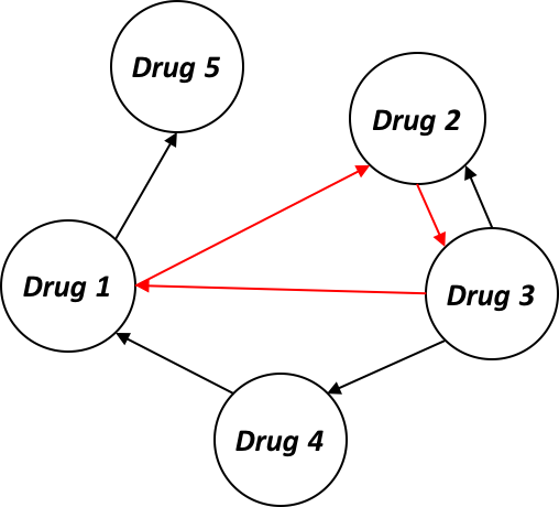
Figure 1. (a) A collateral sensitivity map: This map represents the results of a hypothetical experiment in which tumors are exposed to one drug (row), and after resistance to this drug develops are tested against another drug (column). The color is then the change in sensitivity from the wild type to the evolved strain. (b) A collateral sensitivity network showing every drug pair and their collateral sensitivity relationship. Nodes represent drugs, and directed edges point from drugs, which when resistance develops, end with sensitivity to another (edge terminus). The three drugs connected by the red arrows is an example of collaterally sensitive drug cycle.

Mathematical Model

The key feature of our model is the way to understand the heterogeneity of tumor cells. In the modeling of the drug cycle of $N$ drugs, we assume that the cells are classified into $N$ subpopulations, $R_1$, $R_2$, … and $R_N$. Each subpopulation, $R_i$ is resistant under $Drug\ i$, sensitive under $Drug\ i-1$ (or $Drug\ N$ if $i=1$), and neutral under any of other drugs. Therefore, we can simulate the patterns of collateral sensitivity sequences in terms of the resistant cell populations (for example, $R_{i-1}$) under a particular drug (i.e., $Drug\ i-1$ in the example) which subsequently declines under the next drug in the cycle to which it is sensitive (i.e., $Drug\ i$). (Figure 2).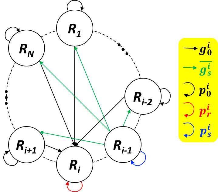

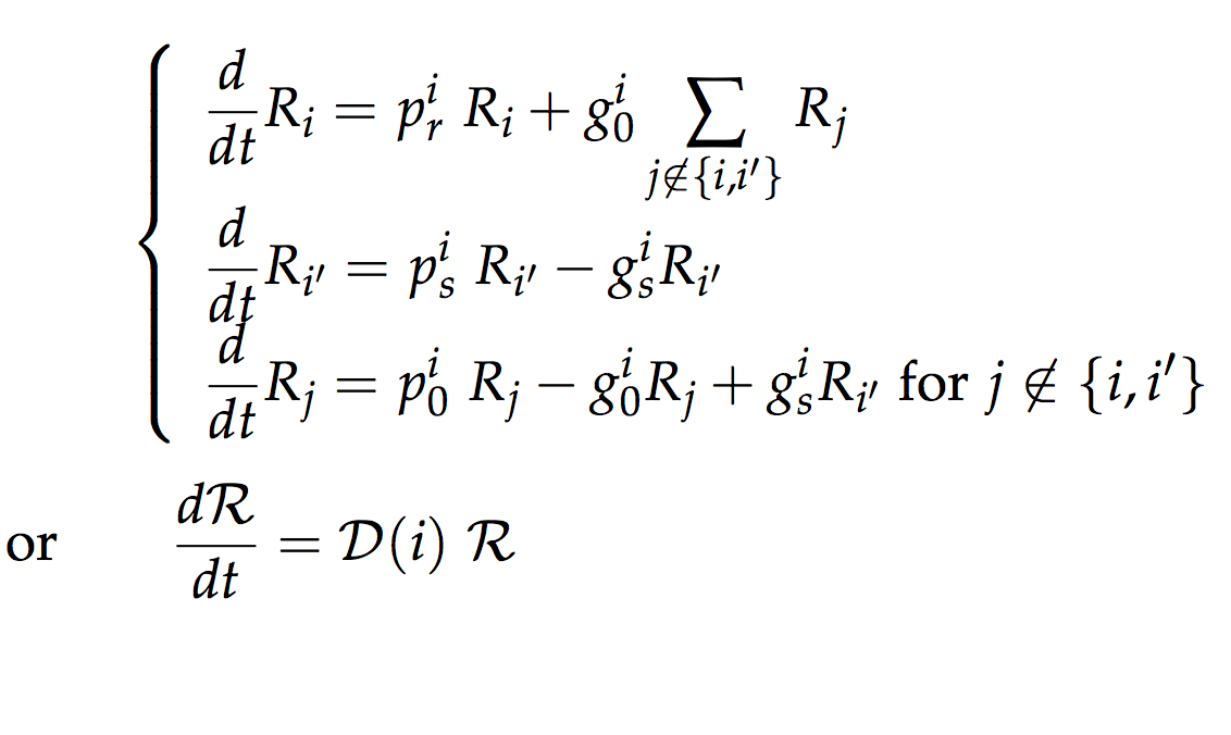
Figure 2: Population dynamics under $Drug \ i$ therapy.

Our cell classification structure does not account complexity of cell compositions beyond the $N$ types of cells, temporally changing collateral sensitivity, any interactions between cells, and so on. However, it could be still meaningful in that it reflects collateral sensitivity phenomena reasonably and the simplicity of the corresponding linear ODE system enables analytic study.

Optimal therapy

Based on the model just introduced, we found the optimal therapeutic strategy to reduce cancer size. The optimal scenario can be achieved when we choose the best drug among the $N$ drugs in terms of the ability to decrease total cell population every moment³, which can be expressed by:

\begin{equation} \frac{d\mathcal{R}}{dt}=\mathcal{D}\left(\underset{1 \leq i \leq N}{\operatorname{argmax}} \ \text{ effect of }Drug\ i\text{ at } t \right) \ \mathcal{R}. \end{equation}
This is an abstract strategy of treatment, as it involves unrealistic instantaneous drug change. However, we can approximate the behavior under the strategy by a piece-wise continuous differential system with drug selection on discrete time points. An example simulation of the approximated optimal therapy with a cycle of 4 hypothetical drugs ($N=4$) is show on Figure 3. Expectedly, the cell subpopulations, effectiveness levels of each drug, and utilized drug sequences are dynamically changing over the therapy period.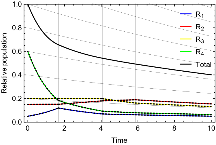

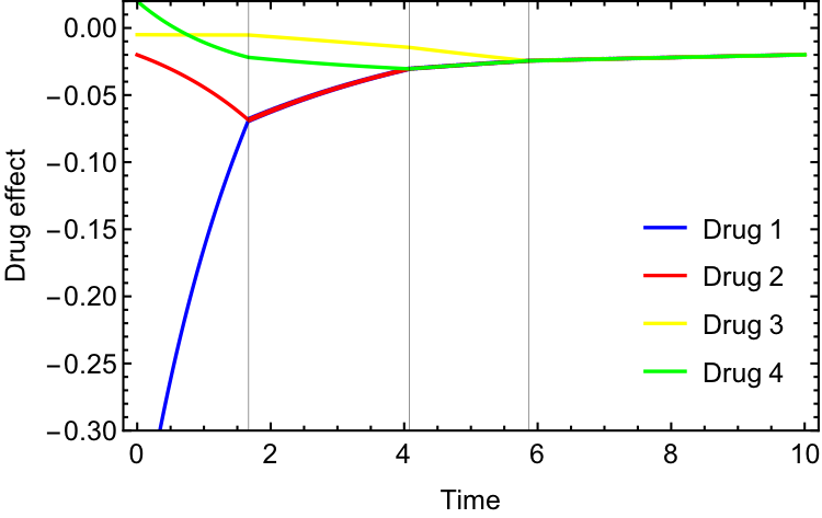
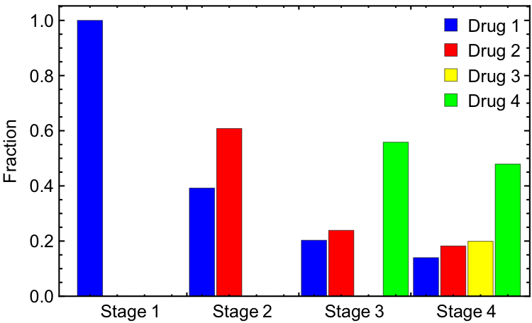
Figure 3: Optimal therapeutic dynamics with a cycle of four symmetric drugs. (a) Histories of subpopulations and total population with gray lines/curves indicating the ends of stages and exponential curves compatible to the last stage. (b) Effects of the drugs (rate of total population change under the drugs) along the optimal population dynamics. (c) Stage-wise relative frequencies of the drugs chosen in the optimal histories simulation.

Based on such numerical simulations, we found that there are (up to) $N$ "stages" of time periods in the optimal administration. We define a stage as a time interval in which a same drug combination is involved. (Example: 3C) Starting initially with the most effective drug(s) of the first stage, with progression to subsequent stages, one or more additional effective drug(s) is chosen to start, and eventually at the last stage all the drugs are activated. All stages except the last one choose better drugs and gradually level the effectiveness of all drugs evenly, so we will call those finite stages the “shaping period”. On the other hand, in the last stage, drugs are equally effective for the shaped heterogeneous tumor, with all drugs being given to continue this balanced effect. Also, the relative subpopulations remain same. Therefore, we will call this stage the “adaptive therapy period”. In the adaptive therapy period, all the subpopulations (and total population) exponentially change with a same exponential rate. (Example: 3A)

The optimal dynamics of cell population (Equation (1)) is equivalent to the following differential system with a finite number ($\leq N-1$) of jump discontinuity that occurs at a "Stage" change.

Practical implementation of the optimal therapy

Our next interest is if we can make our theoretical treatment strategy applicable in the clinical environment. For this practical implementation, we developed a discretized algorithm which works without perfect knowledge about the model parameters and tracking certain subpopulations. (Figure 4) The algorithm requires only trackable total population to run. According to our sample simulation, we found that the algorithm can approximate the analytically determined optimal therapy (Equation 2) quite well, depending on the proper choice of the algorithm parameter. (Figure 4) While we realize that these results are only theoretical, we hope that they can stimulate questions about optimal therapy in realistic scenarios, and that our algorithm for data collection can motivate trialists to collect more temporal data.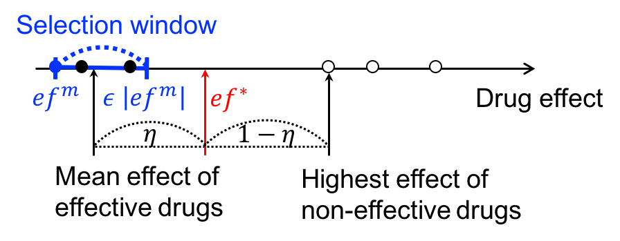

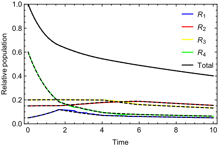
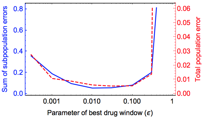
Figure 4: Algorithm and example simulation for the administration of the optimal drug schedules when total population data is available, but not subpopulation nor drug pa- rameters. (a) Diagram of the classification of “effective” and “ineffective” drugs, and the threshold of drug effectiveness (ef∗). The effectiveness levels of the most effective drug (efm), effective drugs and ineffective drugs are indicated by blue-filled circle, black-filled circles and empty circles, respectively. (b) Flow chart of the optimal therapy algorithm based on the “effective” drugs from (a). (c) Comparison between the realistic approximation the optimal therapy generated by the algorithm (b) – solid curves, and the actual one by Equation (1) – dashed curves. ε = 0.03 and η = 0.5 and the other used parameters and initial tumor status are the same as in the example in Figure 3. (d) Errors between the ap- proximated and actual optimal histories, over the range of the parameter of effective drug window.

References

1. A. Dhawan, D. Nichol, F. Kinose, M. E. Abazeed, A. Marusyk, E. B. Haura, and J. G.Scott, “Collateral sensitivity networks reveal evolutionary instability and novel treat-ment strategies in alk mutated non-small cell lung cancer,”Scientific reports, vol.7, no.1,p.1232,2017.
2. N. Yoon, R. Vander Velde, A. Marusyk, and J. G. Scott, “Optimal therapy schedulingbased on a pair of collaterally sensitive drugs,”Bulletin of mathematical biology, vol.80,no.7, pp.1776–1809,2018.
3. N. Yoon, N. P. Krishnan, and J. G. Scott, “Modeling of collaterally sensitive drug cycles,and optimization of the drug effect in the spirit of adaptive therapy,”bioRxiv,2020.