---

Preface

The evolutionary public goods game (PGG) is used to address open questions that arise from facultative contributions of benefits into common spaces, for example in economics, behavior, the evolution of cooperation and more recently, it has been used in the context of cancer to explain the emergence and maintenance of heterogeneity. In our previous paper at Nature communications biology³, we described the importance of nonlinear public goods games to describe the conditions needed for heterogeneity to be maintained (link to blog post). Our paper published in PLoS Computational Biology in 2019 discussed the impacts of spatial heterogeneity in the context of a PGG with two strategies: producers and defectors. The producers made the public good, both types used it to increase their net growth rate. Given similar biological parameters, we showed that spatial effects were quickly removed as the homogeneous stable state winner quickly dominated if the two types were randomly spread out. However, when there was clear separation, the dominant type would travel across the domain with a certain speed. We define a domain to be a space on which the population in question is permitted to grow. The calculation of this speed and its sensitivity to biological parameters is important in the discussion of infiltration of cancer cells through tissue.

Infiltration into nearby tissue is a hallmark of disease progression in cancer. The rate at which cancer cells migrate can then be a useful prognostic tool for understanding disease stages. In addition, finding ways to control this migration rate by altering the tumor micro-environment could be used therapeutically to improve treatment outcomes by minimizing disease spread.

Therefore, understanding the biological system that governs the speed at which cells move into unoccupied space is warranted. From a simplified view, the effect of cancer spreading outward takes the form of a traveling wave. A classic tool for understanding these waves is using the Fisher-Kolmogorov-Petrovsky-Piskunov (F-KPP) equation (wow that is a mouthful!).

Before diving into the rich history of the F-KPP, I would first like to motivate it by appealing to those familiar with population growth. The logistic model $$ \begin{equation} \dot n = r n \left(1 - \frac{n}{K} \right) \end{equation} $$ has been used for over 150 years to describe population dynamics of cells¹, cancer^2,3, animals⁴, and people⁵. In (1), $r$ denotes the growth rate and $K$, the maximal capacity that the environment can contain.

Equation (1) can be thought of as a well-mixed model. That is, a population whose spatial dynamics can be neglected. This can happen when the time scale on which movement or migration occurs is much more rapid than the time scales involving replication.

A method ubiquitous in science, a complicated process is first broken up into simpler parts and then more complex dynamics are slowly reintroduced. Sometimes this leads to minimal changes. Other times, new phenomenons arise. A natural extension to (1) is to include the spatial effects that were originally neglected. A common way to introduce spatial effects is to include a diffusion term. The result is the famous F-KPP equation: $$ \begin{equation} \dot u = D \nabla^2 u + r u (1 - u), \end{equation} $$ where we have defined $u = n/K$ to simplify the notation. The diffusion term creates random motion that causes the population density $u$ to spread out evenly through the domain over time. Other modifications to include spatial effects (e.g. directed motion, chemotaxis) exist as well⁶.

More general forms of (2) can be introduced that are more problem specific. A recent paper written in collaboration with experiments has been helpful in obtaining analytical estimates for the infiltration speed of cancer cells in vitro⁷.

Fisher-Kolmogorov-Petrovsky-Piskunov (F-KPP) equation

The F-KPP falls under a general class of partial differential equations (PDEs) known as reaction-diffusion equations. Analyzed during the 1930s, Fisher, a famous statistician considered the infiltration of advantageous genes through a spatially segregated domain⁸.

Around the same time, Kolmogorov, Petrovsky and Piskunov (KPP) also arrived at (2) when discussing the movement of advantageous genes⁹. However KPP derived the equation using first principles to arrive at an equation that was functionally comparable to (2).

The F-KPP equation has become ubiquitous to many areas of science, ranging from biology¹⁰ and chemistry¹¹, to pure areas of mathematics¹². Perhaps the most well-studied phenomenon of F-KPP, are the traveling-wave solutions and the conditions that allow these traveling-waves to form. For $r > 0$, it can be shown that for certain initial conditions (e.g. In 1D $u(x,t)$ with $u(x,0) = H(x - L/2)$ where $H(x) = 1$ if $x \ge 0$, and 0 if $x < 0$) admits a traveling wave solution $u(x,t) \to U(x - \eta t)$ with speed $\eta$ to be found.

To see this, we start from equation (2) with the above Ansatz and obtain $$ \begin{equation} 0 = DU'' + \eta U' + r U(1-U). \end{equation} $$ The unstable steady state is $U = 0$ and the stable state is $U = 1$. Linearizing about $U = 0$ results in $0 = DU'' + \eta U' + rU$, from which it can be shown that the minimum achievable speed is $\eta = 2 \sqrt{r D}$. This is speed predicted from linear theory. This turns out to be the speed that waves approach under many conditions¹².

Yet another approach for analyzing the behavior of the wave speed $\eta$ involves a form of dimensional analysis. Appeal to (3), but introduce a rescaling of the derivative by a factor $\alpha$, to be determined. This leads to: $$ \begin{equation*} 0 = D\alpha^2 U'' + \alpha \eta U' + rU(1-U). \end{equation*} $$ Lets choose $\alpha$ so all terms are of the same order. This leads to $D \alpha^2 \sim \alpha \eta \sim r$. The first and second implies that $\eta \sim D \alpha$ and the first and third imply that $\alpha \sim \sqrt{r/D}$. Therefore $\eta \sim \sqrt{r D}$, which is the same as the analytically predicted speed up to a constant.

When the wave profile and speed is properly captured by linear theory, the waves are known as "pulled" waves. Often though, the wave profile and speed is not captured by linear theory, and is dependent on the full nonlinearity. These are known as "pushed" waves and are much more difficult to analyze and so we typically resort to numerical methods.

Simulating the wave and calculating its speed

The prediction of the wave speeds offers insight into the infiltration rate of cancerous cells through tissue. However, the typical analytical wave speed prediction is predicated on the fact that the speed is governed by linear theory discussed in the previous section (see gif for convergence to predicted wave speed as the wave travels across the domain). When this property does not hold, the wave speed can be difficult, if not impossible to predict analytically. Instead, we must resort to numerical methods. Standard practice has been to solve (2) on an "infinite" domain (e.g. of size $L$ where $L$ is sufficiently large, such that boundary effects can be neglected). After waiting a sufficient amount of time so the wave has properly formed, one tracks the location of a unique point in the wave (e.g. $u(x,t) = 1/2$). By tracking this point, and recording it, one has the approximate speed of the wave given by $$ \begin{equation} \eta = \frac{x(u = 1/2,t + \Delta t) - x(u = 1/2, t)}{\Delta t}. \end{equation} $$ This method has three main drawbacks. First, it requires a large domain on which we can safely say boundary effects have been neglected. Secondly, there is the inherent difficulty in deciding when the wave has "formed". Third, discretization introduces numerical errors, which cause the wave to constantly reform its shape.

An alternative speed calculation method

We propose an alternative method to calculating the wave speed that exploits the fact that domains in reality are finite. Rather than try to avoid the boundary effects, we will embrace them.

The method is justified semi-rigorously in our recent work by appealing to differences in behavior at different length scales¹³. Put simply, where a traveling-wave solution is admissible, the wave will begin to form and move (possibly concurrently). Once formed, it will rapidly approach its wave speed. This wave can be sometimes be calculated by linear theory (pulled), but is more difficult when it cannot. These waves are known as "pushed". Next, the wave will approach the boundary and will begin to equilibrate to the stable steady state. When the solution is within a predefined exit criterion of the spatially homogeneous steady state, we exit and report the time $\tau$.

Mathematically, the time $\tau$ can be split into three components $$ \begin{equation} \tau = \tau_{\text{wave formation}} + \tau_{\text{wave propagation}}(d) + \tau_{\text{boundary}}(\vec u), \end{equation} $$ where $\vec u$ is the spatially averaged value "close" to the boundary and $d$ is the distance traveled. We also know that the wave propagation term is proportional to the length of the domain. The key insight now is to recognize that we can take two lengths $L_1$ and $L_2$, compute $\tau_1$ and $\tau_2$, the resulting difference will contain only the wave propagation term. This occurs because the behavior of the boundary and the wave formation details are unchanged due to the size of the domain (provided that the domain is sufficiently large that at least some time is spent in the wave propagation phase).

After rearrangement (and noting that $\tau_{\text{wave propagation}}(d) = d/\eta$), we arrive at a result which bares a striking resemblance to (4) $$ \begin{equation}\label{eq:new method} \eta = \frac{d_2 - d_1}{\tau_2 - \tau_1} = \frac{\Delta d}{\Delta \tau}. \end{equation} $$ However, the similarity ends at form. Equation (6) is a large improvement in the standard method for calculating the wave speed.

It can be shown (see footnote 1) that our method is first-order accurate in time and space, with accuracy improving with finer discretization or faster wave speeds: $$ \begin{equation} \eta_{\text{predicted}} = \eta_{\text{actual}} \left[ 1 + \eta_{\text{actual}}^{-1} \mathcal O(\Delta t,\Delta x) \right]. \end{equation} $$

Comparing the two methods

Clearly the standard method (4) should only be used when sufficiently far from the boundary. It is clear that the further away from the initial condition we are, the more accurate (4). So to compare the methods, we will look at the wave speed predictions for a given $L$ starting from a step condition at $x = L/2$. We will take the speed at $x = 3L/4$ and compare with linear theory and (6), where we will take only the smallest two lengths. The result (figure 1), clearly shows the improvement of (6) over the standard method (4).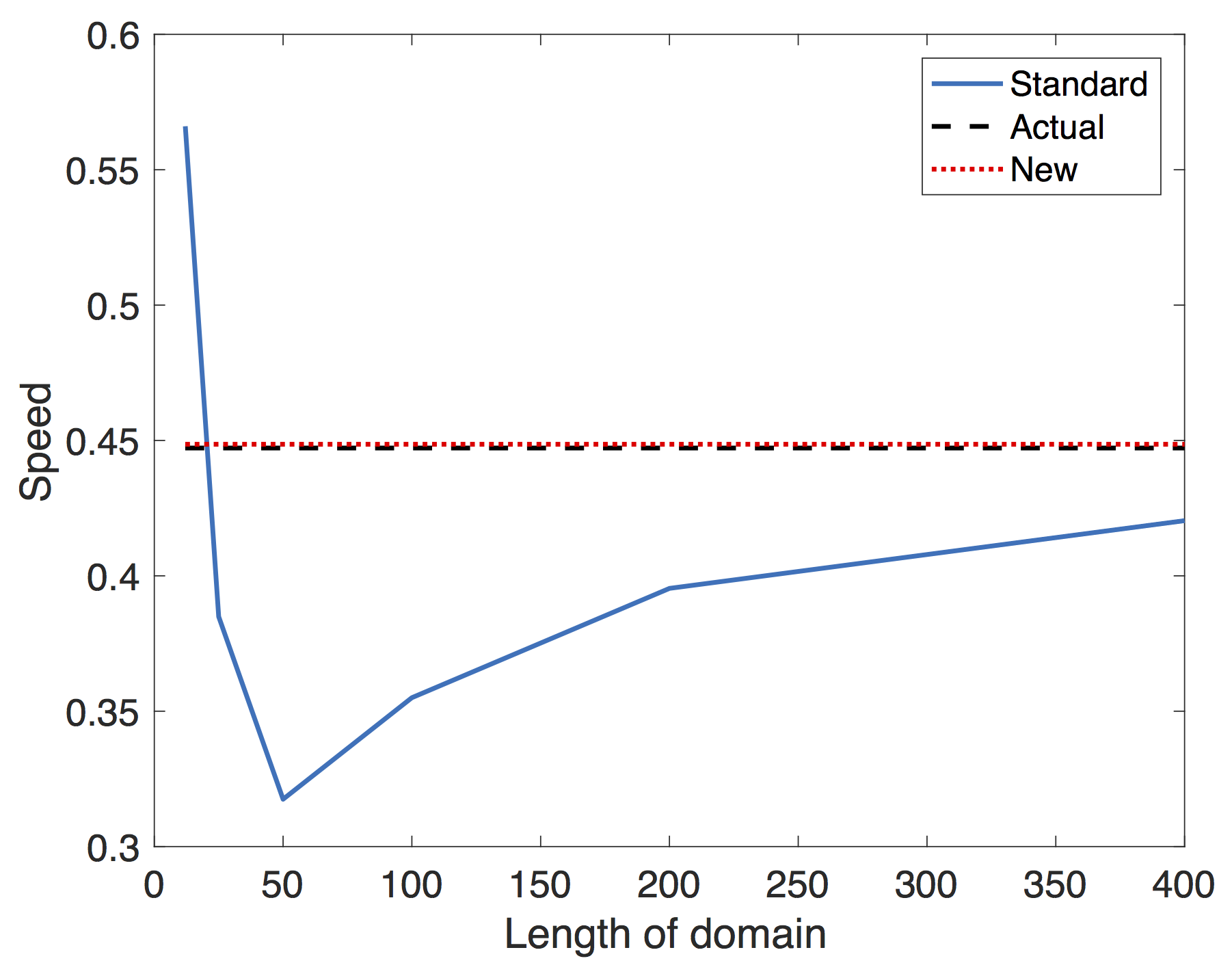

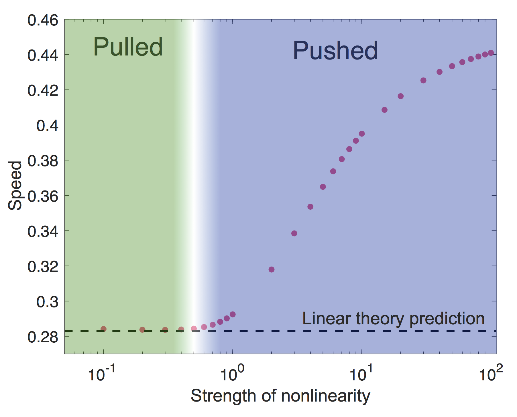
Figure 1: A: The estimated wave speed using (4) (solid,blue) and (6) (dotted, red). As expected, the standard method begins to converge to the true wave speed, but requires a very large domain. In contrast, (6) is accurate using even the smallest two sizes $L = 12,25$. The predicted wave speed $\eta_0 = 2\sqrt{rD} \approx 0.447$ with $r = 0.05$ and $D = 1.0$. B: Our method gives a robust way to distinguish that a transition to nonlinear wave speeds are occurring and that it is not a domain size issue. (adapted from ref. 13).

The size of the domain needed for the standard method to give accurate results depends strongly on the wave shape as well as the speed. Slower waves, will have more time to properly form, but typically involve higher resolution, a shortcoming not observed with the new method. In figure 2, we see that speed approaches the theoretical speed, but only near the end of the simulation where we also see the calculation begin to give false results as it hits the boundary $(L = 50)$. Further, oscillations in the wave speed prediction are common as we are restricted by the discretization of the domain. We took $\Delta t = 0.01$ and $\Delta x = 0.1$. The relative error ranged from 0.7% - 2.3%. The situation is worse for $L = 25$ which ranged from 3.23% - 4.65%. In contrast taking $L = 25$ and $L = 50$, with $r = 1, D = 0.1$ results in a relative error of 1.41%.

Figure 2: Wave speed calculation as the wave forms and moves through the domain. The speed asymptotes to the predicted wave speed as it approaches the proper wave form.

Conclusion

We have shown that the new method (6) outperforms the standard method and at worst gives comparable results. The ability to predict the wave speed accurately, without having to resort to large domains, offers the ability for computational speedup in order to gain insight into which parameters are most sensitive in controlling the speed of infiltration.

From this we could design experiments to test whether altering these biological parameters can slow down cancer cell infiltration and thus slow disease progression.

Footnotes

1. To see this, let $\eta_0$ be the true wave speed in the limit $\Delta t, \Delta x \to 0$. Taylor expanding the terms in (5) with two different lengths with $h, k \ll 1$, we have $$ \begin{align*} \tau^{(1)} & = \tau_0^{(1)} + \left(h \frac{\partial \tau^0_{WF}}{\partial h} + k \frac{\partial \tau^0_{WF}}{\partial k} \right) - \frac{d^{(1)}}{\eta_0^2} \left(h \frac{\partial \eta_0}{\partial h} + k \frac{\partial \eta_0}{\partial k} \right) + \left(h \frac{\partial \tau^0_B}{\partial h} + k \frac{\partial \tau^0_B}{\partial k} \right) \\ \tau^{(2)} & = \tau_0^{(2)} + \left(h \frac{\partial \tau^0_{WF}}{\partial h} + k \frac{\partial \tau^0_{WF}}{\partial k} \right) - \frac{d^{(2)}}{\eta_0^2} \left(h \frac{\partial \eta_0}{\partial h} + k \frac{\partial \eta_0}{\partial k} \right) + \left(h \frac{\partial \tau^0_B}{\partial h} + k \frac{\partial \tau^0_B}{\partial k} \right) \\ \Delta \tau & = \Delta \tau_0 - \frac{\Delta d}{\eta_0^2} \left(h \frac{\partial \eta_0}{\partial h} + k \frac{\partial \eta_0}{\partial k} \right) \\ \frac{1}{\eta} & = \frac{1}{\eta_0} \left[ 1 - \frac{1}{\eta_0} \left(h \frac{\partial \eta_0}{\partial h} + k \frac{\partial \eta_0}{\partial k} \right) \right]. \end{align*} $$ (jump back)

References

1. Daniel A Charlebois and Gabor Balazsi. Modeling cell population dynamics. In silico biology, 13(1-2):21–39, 2019.
2. Matthew D Johnston, Carina M Edwards, Walter F Bodmer, Philip K Maini, and S Jonathan Chapman. Mathematical modeling of cell population dynamics in the colonic crypt and in colorectal cancer. Proceedings of the National Academy of Sciences, 104(10):4008–4013, 2007.
3. Gregory J Kimmel, Philip Gerlee, Joel S Brown, and Philipp M Altrock. Neighborhood size-effects shape growing population dynamics in evolutionary public goods games. Communications biology, 2(1):1–10, 2019.
4. LM Cook. Oscillation in the simple logistic growth model. Nature, 207(4994):316–316, 1965.
5. Pierre-Fran ̧cois Verhulst. Notice sur la loi que la population suit dans son accroissement. Corresp. Math. Phys., 10:113–126, 1838.
6. James D Murray. Mathematical biology: I. An introduction, volume 17. Springer Science & Business Media, 2007.
7. Gregory J Kimmel, Mark Dane, Laura M Heiser, Philipp M Altrock, and Noemi Andor. Integrating mathematical modeling with high-throughput imaging explains how polyploid populations behave in nutrient-sparse environments. Cancer Research, 80(22):5109–5120, 2020.
8. Ronald Aylmer Fisher. The wave of advance of advantageous genes. Annals of eugenics, 7(4):355–369, 1937.
9. AN Kolmogorov, IG Petrovsky, and NS Piskunov. Investigation of the equation of diffusion combined with increasing of the substance and its application to a biology problem. Bull. Moscow State Univ. Ser. A: Math. Mech, 1(6):1–25, 1937.
10. Oskar Hallatschek. The noisy edge of traveling waves. Proceedings of the National Academy of Sciences, 108(5):1783–1787, 2011.
11. Gyorgy Bazsa and Irving R Epstein. Traveling waves in the nitric acid-iron (ii) reaction. The Journal of Physical Chemistry, 89(14):3050–3053, 1985.
12. Wim Van Saarloos. Front propagation into unstable states. Physics reports, 386(2-6):29–222, 2003.
13. Gregory J Kimmel, Philip Gerlee, and Philipp M Altrock. Time scales and wave formation in non-linear spatial public goods games. PLoS computational biology, 15(9):e1007361, 2019.