---

Five years ago, we published a preprint titled "Antifragile therapy," wherein we described the concept of antifragility, and how it might apply to cancer therapy [1]. The concept was very simple: a fragile system is one that is harmed by perturbations, and an antifragile system is one that benefits by perturbations. The concept readily applies to cancer therapy. Oncologists can perturb the tumor ecosystem via cancer therapy. We've long known that the dose makes the poison [2], but we now also know that dose timing can make or break the effect (see footnote 1).

Five years ago, we sought to assess whether the mathematical framework of antifragility can be applied to cancer therapy. Antifragility intercepts conceptually with the idea of intermittent therapy, which introduces drug holidays to slow resistance evolution (see for example, ref. [3]). We view this as a dose 'perturbation' where the timing of dose perturbations (or lack thereof, in terms of treatment holidays) can improve therapeutic effectiveness. So, why the long gap between the first manuscript in 2020 and this new preprint, in 2025?

Two reasons: one is a mathematical problem and the second is an evolutionary problem.

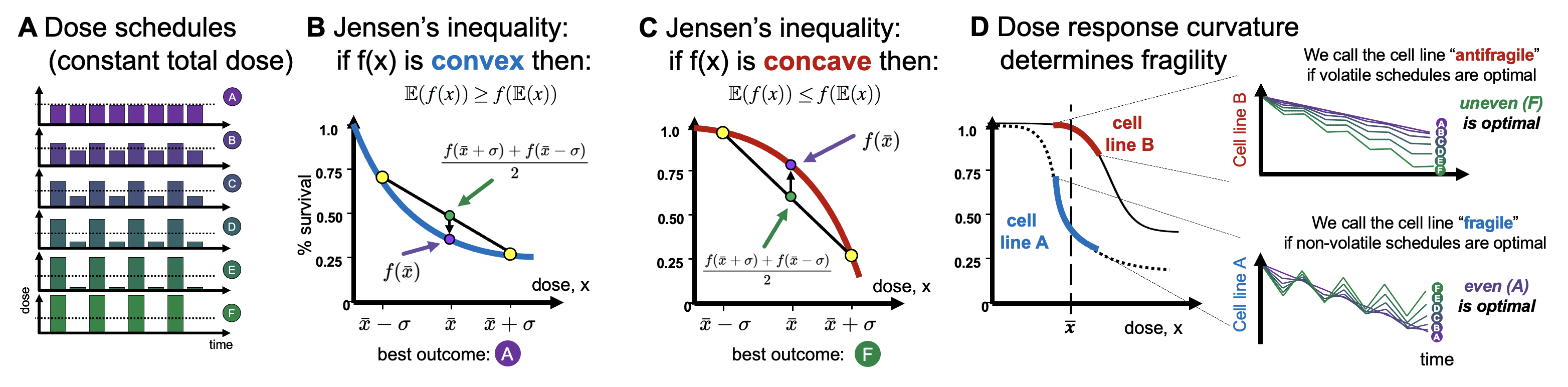
1. The mathematical problem

If the dose response function is known, it is straightforward to compare continuous dosing with an intermittent dosing schedule (see figure 1A). The response to various treatment schedules depend on the convex (figure 1B) or concave (figure 1C) or concave-convex (figure 1D).

Consider a cycle of treatment: \begin{eqnarray} \texttt{Treatment Cycle} = \{\bar{x} + \Delta, \quad \bar{x} - \Delta\} \label{cycle_eqn} \end{eqnarray} where $\bar{x}$ represents the dosing schedule's mean dose value and $\Delta$ represents the dosing schedule's variance. In this way, all treatment schedules have identical dose mean, enabling us to compare second-order effects that are due to alterations in variance only. We term a dosing schedule "even" (purple in figure 1A) if there is no variance ($\Delta = 0$) or "uneven" (green in figure 1A) if the variance is non-zero ($\Delta > 0$).

For example, compare the effect of a dose, $x$, to an alternative dosing schema of 120% $x$ followed by a lower dose of 80% $x$. If the dose response is convex, we expect: \begin{equation} \frac{f(x+\Delta)+f(x-\Delta)}{2} > f(x) \label{jensens_two_dose} \end{equation} The left-hand side is the average (indeed, the expectation, $\mathbb{E}(f(x))$) of two dose effects, while the right-hand side is the function evaluated at the average dose, or $f(\mathbb{E} (x ))$. This is illustrated in figure 1B, where the right-hand side is marked with a purple circle while the left-hand side is marked with a green circle, denoting the average of the high and low doses (green circles). If the dose-response is concave, the inequality is flipped, and the purple circle is above the green circle.

The inequality above will flip if the dose response is concave (see footnote 2).

So, what's the mathematical problem? Determining the appropriate metric for $f(x)$. Consider the following figure. What is the appropriate metric for describing the dose response function, $f(x)$? Should it be log-linear, linear-linear, linear-log, or log-log? Visually, this obviously changes the convexity (or concavity) of the dose response curve, so it's unclear which option is appropriate.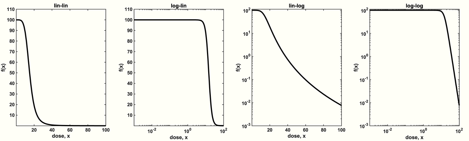

Solving the mathematical problem

To answer the question, we begin by considering a population of tumor cells under treatment with initial size $n_0$ and growth rate $\gamma(x)$ the final size, $n$, is given by: \begin{eqnarray} n(T) = n_0 \exp(\gamma(x) T ), \end{eqnarray} where $\gamma(x)$ is the rate of growth of the tumor under treatment with dose $x$ over a time interval of $T$. The quantity within the parenthesis is known as the log-kill effect, which we denote by the parameter $\beta(x) = \gamma(x) T$. Thus, the effect of multiple doses can be predicted via a summation of the log-kill effect. \begin{eqnarray} n &=& n_0 \exp\big( \beta(x) +\beta(x)\big) \label{additive_tumor_dynamics}. \end{eqnarray} Next, we assess the effect of variation in the input dose, $x$, by comparing an even (non-volatile) dosing scheme to an uneven (volatile) dosing scheme. \begin{eqnarray*} n_{\texttt{even}} &=& n_0 \exp\big( \beta(x)+\beta(x)\big) \\ n_{\texttt{uneven}} &=& n_0 \exp\big( \beta(x+\Delta) +\beta(x-\Delta)\big) \end{eqnarray*} The definition of antifragility (e.g. eqn.~\eqref{jensens_two_dose}) requires that the effect of each input is additive and independent. The dose-dependent log-kill rate, $\beta(x)$, satisfies both conditions. Thus, it is useful to define a metric of fragility, $F$, to compare the log-kill rate of a tumor under even ($\sigma = 0$) dosing or under uneven ($\sigma > 0$) dosing: \begin{equation} F(x,\Delta) = \beta(x+\Delta)+\beta(x-\Delta) - 2\beta(x). \end{equation} If uneven treatment protocols result in maximizing tumor regression, then it will result in $F<0,$ and we term this situation antifragile. Conversely, if even dosing protocols result in maximizing tumor regression, $F>0$, it is fragile.

Rearranging some terms, it's straightforward to show the following relation: \begin{equation} F = \ln \bigg( \frac{n_{\texttt{uneven}}}{n_{\texttt{even}}} \bigg) \end{equation} Or, more conveniently: \begin{equation} n_{\texttt{uneven}} = n_{\texttt{even}} \exp (F). \end{equation} Therefore, fragility, $F$, is interpreted as the log-kill gain (or loss) of switching to an uneven treatment schedule, compared to baseline even dosing. Patients will benefit (i.e. maximizing tumor kill) by switching to an uneven dosing protocol when $F<0$.

The appropriate measure of convexity is the exponential growth rate of tumors as a function of dose delivered, $\beta(x)$.

Drug-induced proliferation curves preserve convexity

There are several examples of dose response models that mimic this $\beta(x)$ function above. First, GR-curves plot the exponential growth rate inhibition, normalized by control [4]. Second, drug-induced proliferation curves plot the exponential growth rate, usually converted to units of 'doubling time' [5]. Finally, if you're plotting a simple % survival dose response curve in 72 hours, you can use a log-linear plot to preserve convexity (assuming that growth rate is constant within the time window measured).

2. The evolutionary problem

Next, I'll show a brief teaser of the most exciting result from our recent preprint. Now that we've settled on Drug-Induced-Proliferation (DIP) curves as the appropriate metric for measuring convexity (and thus, antifragility) - we apply it to ALK+ non-small cell lung cancer. It so happens that ALK inhibitors have a convex dose response (see figure 3A), and thus continuous therapy minimizes tumor growth.

Through math modeling, we also measured the rate of resistance. It so happens that ALK inhibitors have a concave shaped function that describes the rate of plastic resistance as a function of dose. The evolutionary 'problem' is that dose response curves are not static - they evolve in response to selection pressures.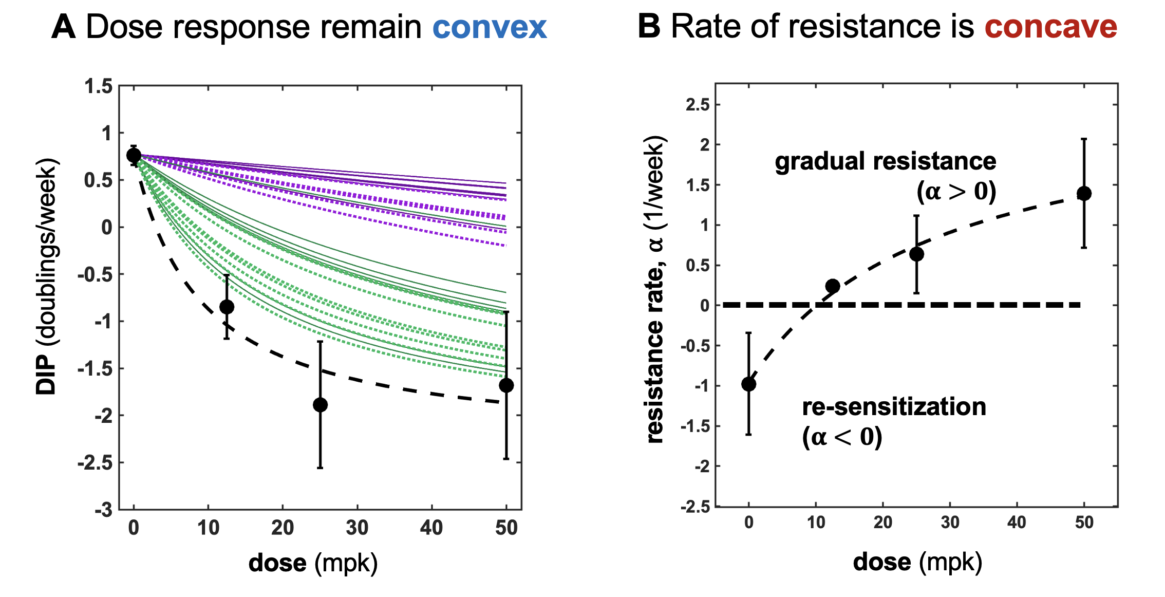

But this evolution of resistance induces an exciting trade-off between convex tumor response and concave tumor resistance. This is why we titled the manuscript "Evolutionary Antifragile Therapy" - to illustrate the connection to Evolutionary Therapy. In the manuscript, we explore several alternative protocols that aim to minimize tumor growth and minimize resistance, such as switching to intermittent dosing after a prolonged period of continuous dosing (or vice versa). Future work will address the connection to adaptive dosing schema, which are not a prior fixed dosing schedules, but adaptive protocols based on tumor response. In this way, the long-term vision is to think of antifragility as a conceptual (and mathematical) tool in the broad toolset of evolution-based treatment strategies.

Footnotes

1. The original quote was apparently written by Paracelsus in 1538, writing "Alle Dinge sind Gift, und nichts ist ohne Gift; allein die Dosis macht, dass ein Ding kein Gift ist." or, "All things are poison, and nothing is without poison; the dosage alone makes it so a thing is not a poison. (jump back)

2. This contrived example can be extended to weigh the effect of the two uneven doses by the time spent on the dose: \begin{equation} \lambda f(x+\Delta)+ (1-\lambda)f(x-\Delta) > f(x), \end{equation} where $0\geq \lambda \geq 1$. Previously, eq.~\ref{jensens_two_dose} is a special case for $\lambda =0.5$. The math can also be extended to consider an arbitrary number of doses, whose effect is weighted (\(\lambda_i\)) by the length of time of that dose. Thus, it's straightforward to arrive at the following general definition: \begin{equation} \sum_i^{N} \lambda_i f(x_i) > f \left ( \sum_i^N \lambda_i x_i \right) \label{discrete_antifragility} \end{equation} where each $\lambda_i$ value is a weight such that $\lambda_i \in [0, 1]$ and $\sum_i \lambda_i = 1$. (jump back)

References

1. West, J., Desai, B., Strobl, M., Pierik, L., Velde, R.V., Armagost, C., Miles, R., Robertson-Tessi, M., Marusyk, A. and Anderson, A.R., 2020. Antifragile therapy. BioRxiv, pp.2020-10.
2. Die dritte Defension wegen des Schreibens der neuen Rezepte, Septem Defensiones 1538. Werke Bd. 2, Darmstadt 1965, p. 510
3. Kavran, A.J., Stuart, S.A., Hayashi, K.R., Basken, J.M., Brandhuber, B.J. and Ahn, N.G., 2022. Intermittent treatment of BRAFV600E melanoma cells delays resistance by adaptive resensitization to drug rechallenge. Proceedings of the National Academy of Sciences, 119(12), p.e2113535119.
4. Hafner, M., Niepel, M., Chung, M. and Sorger, P.K., 2016. Growth rate inhibition metrics correct for confounders in measuring sensitivity to cancer drugs. Nature methods, 13(6), pp.521-527.
5. Meyer, C.T., Wooten, D.J., Paudel, B.B., Bauer, J., Hardeman, K.N., Westover, D., Lovly, C.M., Harris, L.A., Tyson, D.R. and Quaranta, V., 2019. Quantifying drug combination synergy along potency and efficacy axes. Cell systems, 8(2), pp.97-108.