---

Analysis of a computational model is very important both for its development and for drawing insight from it. During model development, analyses are used to determine which parameters need to be fit to experimental data and which parts of the model could benefit from expansion or reduction. Afterwards, various analyses are used to explore how the model behaves in different regions of parameter space and how different perturbations impact model simulations. For all analyses, two questions that must be asked are “What are the model outputs?” and “How can we compare these outputs?” Aside from the simplest of models, simulations produce outputs that can become very complex and difficult to compare, with only very basic parts of output space (such as the peak of one or two time-courses) serving as the subjects of analysis^1-3. In reality, the outputs are intertwined, and their relationships must be accounted for when comparing simulations. This leads to the issue of being able to account for all of these relationships without introducing bias from the researcher.

In our recent preprint entitled “Siamese neural networks for a generalized, quantitative comparison of complex model outputs”, we developed an approach to holistically compare model simulations without the need to specify a comparison metric. This method accounts for how model outputs are related, including relationships that would be impossible to manually calculate. We do this by using Siamese neural networks⁴ to project model simulations into low-dimensional space and then take the distance between projected simulations, giving us a single, continuous value that answers the question “How different are these simulations?” (Figure 1). This distance can be used as for many different types of model analyses and, when combined with specific outputs of interest, allows us to draw great insight into the modeled system. We tested this approach on several disparate types of models, changing only the neural network structure, showing that this one approach has broad applicability.

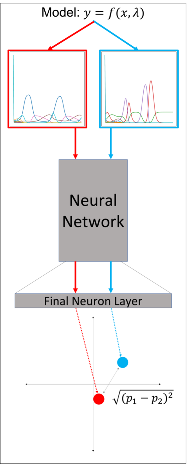
Figure 1: Overview of using a Siamese neural network to project a pair of simulations into low-dimensional space. Taking the distance between projected points provides a metric for determining the similarity between simulations. The smaller the distance, the more similar they are.

The first step of this approach is to produce a training dataset for the Siamese network. We do this by randomly sampling from a uniform distribution for each parameter that we may want to vary, over the widest range that we would want to vary it, producing a set of Monte Carlo simulations. We use this dataset to train the Siamese network via triplet loss⁵, which compares the distance (D) between projected points for an anchor (A) and positive (P) sample to the distance between A and a negative (N) sample, aiming to minimize D(A,P) and maximize D(A,N). To obtain A, P, and N, we randomly select two simulations to be A and N. P is then generated by adding Gaussian noise to A. Many triplets are randomly formed, which are then used to train the Siamese network.

Once we have trained the Siamese network, we can perform a number of different analyses with it. The first example we show is with a four-species Lotka-Volterra model, with the base parameters tuned to create oscillatory behavior⁶. We perform a sensitivity analysis, comparing the sensitivity ranking obtained when using the distance calculated by a Siamese network to the change in a specified sensitivity output, the traditional way of performing sensitivity analysis (Figure 2). Parameters are then ranked by their sensitivity. We see that there are some discrepancies in the ranked parameters, due to the fact that a specified output only looks at a small region of output space, while the Siamese network accounts for the entire output.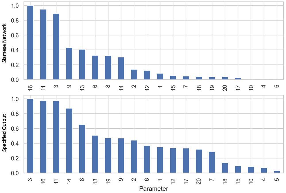

Figure 2: Comparison of using a Siamese network to using a specified output for a sensitivity analysis. Sensitivities are normalized to the highest value. We see that while some parameters are ranked similarly, other parameters are ranked very differently. This is due to the differences in how the sensitivity output is measured.

Lastly, we show an example of applying our approach to an agent-based model of tumor-immune interactions⁷. These models are stochastic and produce complex spatial outputs. Here, we examine the final spatial layout of the simulation. Rather than just calculating the distance between two simulations, we instead use the Siamese network to project the Monte Carlo simulations into low-dimensional space, allowing us to easily cluster the simulations (Figure 3). From this, we can then examine the distributions of the parameters for each cluster, drawing insight on how different tumor properties can yield different end-states. Additionally, we can examine the distributions for specific model outputs, giving us further insight beyond the low-dimensional projections performed by the Siamese network.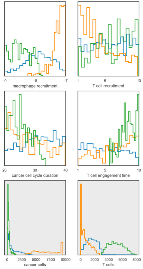

Figure 3: Distributions for parameter values (top two rows) and specific outputs (bottom row) for clustered model simulations.

Our approach facilitates a holistic comparison of model simulations, accounting for the complex relationships between outputs without having to specify a comparison metric. This is similar to the work by Tapinos and Mendes⁸, with the distinction that our method is not limited to model outputs in the form of time-series. Our approach can be used on disparate model types and applied in various different types of analyses. We hope that this approach provides researchers with another way to explore their models in further detail.

References

1. Campbell, K., McKay, M. D. & Williams, B. J. Sensitivity analysis when model outputs are functions. Reliability Engineering & System Safety 91, 1468–1472 (2006).
2. Lenhart, T., Eckhardt, K., Fohrer, N. & Frede, H.-G. Comparison of two different approaches of sensitivity analysis. Physics and Chemistry of the Earth, Parts A/B/C 27, 645–654 (2002).
3. Li, D. & Finley, S. D. Mechanistic insights into the heterogeneous response to anti-VEGF treatment in tumors. Computational and Systems Oncology 1, e1013 (2021).
4. Chicco, D. Siamese neural networks: An overview. Artificial Neural Networks 73–94 (2021).
5. Hoffer, E. & Ailon, N. Deep metric learning using triplet network. in International workshop on similarity-based pattern recognition 84–92 (Springer, 2015).
6. Vano, J., Wildenberg, J., Anderson, M., Noel, J. & Sprott, J. Chaos in low-dimensional Lotka–Volterra models of competition. Nonlinearity 19, 2391 (2006)
7. Cess, C. G. & Finley, S. D. Multi-scale modeling of macrophage—T cell interactions within the tumor microenvironment. PLoS Computational Biology 16, e1008519 (2020)
8. Tapinos, A. & Mendes, P. A method for comparing multivariate time series with different dimensions. PLoS ONE 8(2): e54201 (2013).