---

As the field of mathematical oncology continues to grow, so does the number of models aimed at predicting novel, potentially optimal, therapy. However, for the sake of patients who may potentially receive mathematically informed treatments one day, it is important that we undergo proper model development practices to ensure that our models have been appropriately trained and validated prior to offering treatment predictions. More importantly, it is imperative that we recognize the limitations of our models and are able to identify those that are truly predictive and those that are not. In our article recently published in the Bulletin of Mathematical Biology¹, we propose a pipeline for developing novel, predictive mathematical models and highlight commonly used shortcuts that can lead to patients being treated with ill-informed, model suggested treatment protocols.

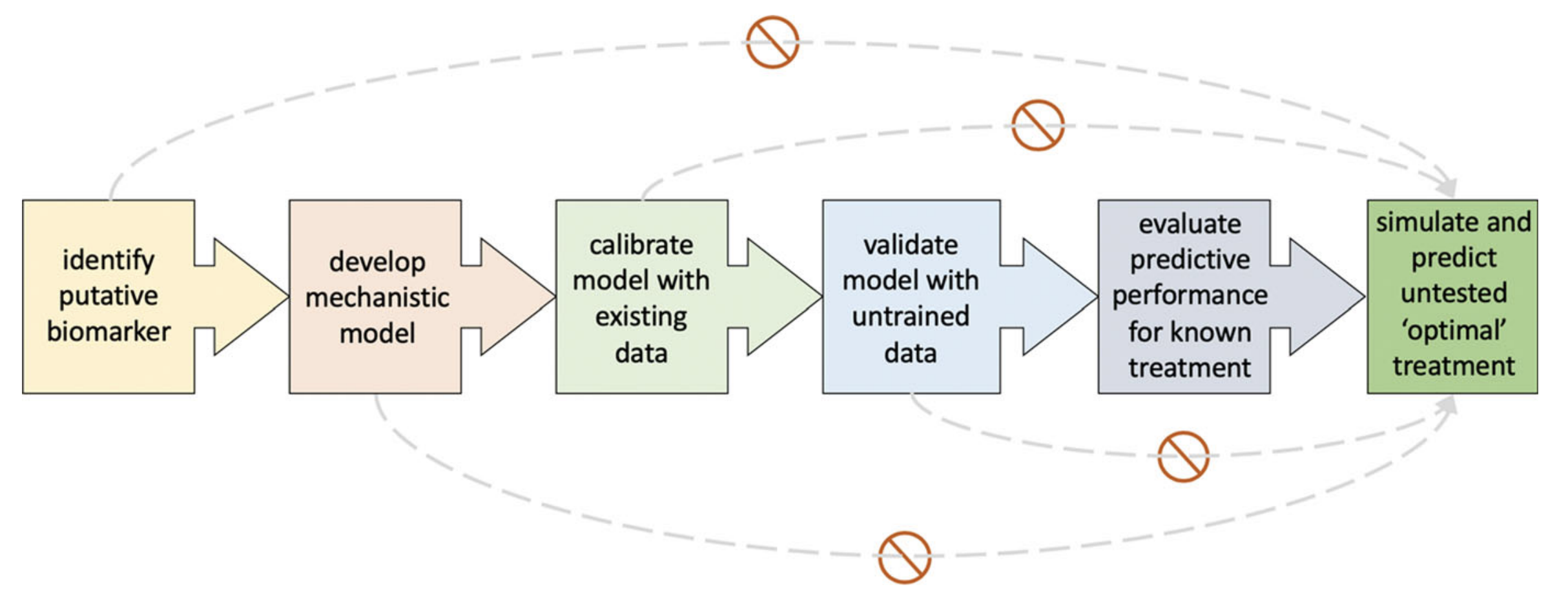
Figure 1: Proposed pipeline for developing predictive models. Grey curves show commonly used shortcuts that should be avoided.

Prior to proposing untested optimal treatment options, a mathematical model should undergo six successive steps (Fig.). First, an appropriate putative biomarker should be identified. This can be the number of circulating tumor cells, tumor volume, or even the tumor’s mutational burden. As predictive models are used to forecast a patient’s response in the future, the biomarker should be dynamic and evolve over time. The second step is to develop a mechanistic model describing the changes in this biomarker over time. The type of model developed, whether an ordinary differential equation model or an agent-based model for instance, will depend on the type of biomarker and the information that it is providing. Once the model has been developed, it should be calibrated to data of responses to known treatments. This will require analyzing individual parameter values to determine the driving forces of the biomarker dynamics. Those parameters driving the dynamics will be patient-specific, while the others can be held uniform across the patient cohort. Model parameterization should be done carefully, ensuring that model parameters taken from literature are not mixing cancer types, experimental conditions, and scales. Proper calibrations will differentiate between models that fit all data and propagate the dynamics forward in time and truly predictive models that use individual changes in biomarker dynamics to inform how the system will evolve over time. It is also important to note that though they are often used interchangeably, model fitting and predicting are distinct and one should not be confused with the other.

After the model has been appropriately calibrated to existing data and the mechanisms driving treatment response have been identified, these finding should be validated in an independent cohort. The uniform parameter values derived during the calibration step should be kept constant, while patient-specific values are found for the other parameters. The next step is to test the model’s ability to predict a known treatment protocol. Once the predictive performance has been evaluated and found to be sufficient, then the model can be used to simulate and predict unknown treatment protocols. It is important that model simulations only include treatment for which the model has been trained on. Also, clinical feasibility as well as possible toxicity should be considered when proposing alterative protocols.

Following these steps will ensure that models go through a rigorous process of calibration, validation, and prediction assessment before it is able to predict and propose alternative treatments. Each step serves as a model quality control and should be tested in succession. Unnecessary shortcuts can have dire consequences for the patients we are building our models for. Keeping ourselves and our models honest will help us to continue to gain the trust and respect of clinicians and patients alike. As the number of mathematical models being incorporated into clinical trials and clinical decision-making rises, employing such a standard will ensure that patients are treated with the highest quality care.

References

1. Brady R, Enderling H. Mathematical Models of Cancer: When to Predict Novel Therapies, and When Not to. Bull Math Biol, (2019).