---

Biology's most (and least) popular equation

If asked for an equivalent of the iconic $e = mc^2$ in biology it would be fair to respond with the logistic equation: $$ \begin{equation} \frac{d N(t)}{d t} = r \left(1-\frac{N}{K}\right) N. \label{eq:rKFormulation} \end{equation} $$ Not only is this one of the most well-known equation in biology (and that means something), but it also forms the foundation of many of our theoretical models of population growth and dispersal (e.g. Fisher's equation). However, unlike Einstein's model of the relationship between energy and mass, the logistic equation is probably despised as much as it is loved. This is particularly true for mathematical oncology, where the logistic equation has consistently been shown to perform badly in describing tumour growth (e.g. [10, 2]), yet continues to form part of our basic model building tool set. In this blog post, I want to share some insights I have gained by studying the history and meaning of this equation whilst working on a recent manuscript¹⁵ for my PhD. In particular, I want to show how thinking about turnover can help to address some of the issues with logistic growth, and why turnover in tumours may be more important than one might at first appreciate.

A brief history of logistic growth

The logistic equation was first introduced (and named) by Belgian mathematician Pierre-Francois Verhulst in 1838¹⁶ but was subsequently independently re-discovered by Anderson McKendrick in 1911¹¹, Raymond Pearl and Lowell Reed in 1920¹³, and Alfred Lotka in 1925⁶. All authors had derived the equation as a mathematical model of how a population might self-limit its growth as Thomas Malthus' had described in his famous "Essay on the Principle of Population Growth" ⁹. If we let \(N(t)\) be the density of the population, and assume that individuals reproduce at constant rate, \(r\), then the population will grow as: $$ \begin{equation*} \frac{d N(t)}{d t} = r N \end{equation*} $$ In short: it will grow exponentially until there are more individuals than atoms in the universe. Malthus, who saw this flaw, argued that because of resource limitations no population will grow in this fashion forever. Verhulst, McKendrick, Pearl, Reed, and Lotka recognised that the simplest way to integrate this into the above equation is to say that the population's growth rate decreases linearly with population density (for example, via a Taylor expansion^16,11,13,6). That is: $$ \begin{equation} \label{eq:raFormulation} \frac{d N(t)}{d t} = (r - \alpha N) N, \end{equation} $$ where \(\alpha\) measures the intensity of this 'crowding effect'.

As you will notice this equation has a slightly different form to the \(r\)-\(K\) formulation we are so familiar with today (more on that in a bit). It also does not yet include the \(K\). The \(r\)-\(K\) formulation originated in the 1930s and was first popularised in a textbook by Raymond Pearl¹². Its advantage was that it was conceptually easier to fit to data: \(K\) can be estimated from the saturation point of the population, and \(r\) by fitting a linear model to the log-transformed growth data. It was subsequently picked up by Gause and Witt who developed the well-known isocline analysis of the Lotka-Volterra competition model⁵. As their work rose to fame, so did the \(r\)-\(K\) formulation.

A final important development was the introduction of the \(r\)-\(K\) selection theory by MacArthur and Wilson in 1967⁷. The \(r\)-\(K\) selection hypothesis states that organisms are selected either for their ability to grow (\(r\)) or their ability to compete (\(K\)). It makes sense that Macarthur and Wilson used the two seemingly independent parameters in the logistic growth model to motivate their theory. However, it has been difficult to find species in which \(r\) and \(K\) change independently - an issue which spurred a lot of debate, and eventually resulted in the development of a more wholistic theory of life history¹⁸. Interestingly, as we will see below, some of this debate might have been avoidable if the \(r\)-\(\alpha\) formulation had been used instead.

The devil is in the details

There is an important, but subtle, difference between the original \(r\)-\(\alpha\) form of the logistic growth equation (Equation \eqref{eq:raFormulation}) and the \(r\)-\(K\) formulation (Equation \eqref{eq:rKFormulation}) - and it is not the \(\alpha\). To illustrate this difference we bring Equation \eqref{eq:raFormulation} into the same \(r\)-\(K\) structure: \begin{align*} \frac{d N(t)}{d t} &= r \left(1 - \frac{\alpha}{r} N\right) N, \\ &= r \left(1 - \frac{N}{\hat{K}}\right) N, \end{align*} where \(\hat{K} = r/\alpha\). We see that in the \(r\)-\(K\) formulation the population will saturate at \(K\) and this level is apparently independent of the intrinsic growth rate, \(r\). In the \(r\)-\(\alpha\) formulation the population settles at \(r/\alpha\), so that when we change \(r\), the population's equilibrium value will change too!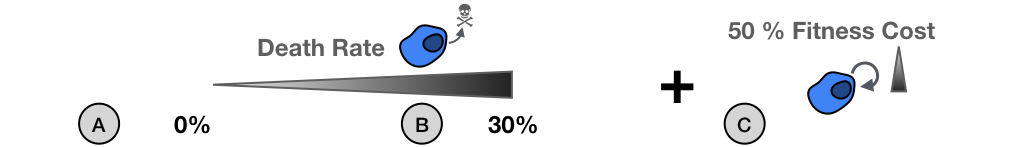

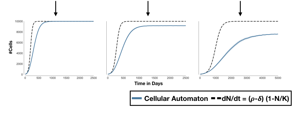
Figure 1: Why \(K\) in the logistic growth model is not just an environmental constraint. A 2-D on lattice, birth-death, cellular automaton model implemented in HAL³. A) No death. Cells proliferate at rate \(\rho=0.027d^{-1}\) until they fill up all 10,000 sites. Setting \(r=\rho\) and \(K=10,000\) in a logistic growth model gives the same predictions. B) With a death rate of \(\delta=30\% \, \rho\) the population can never fully saturate the domain. Only changing \(r\) in the logistic growth fails to capture this. C) Reducing \(\rho\) by 50% further decreases the number of cells at equilibrium. Again this is missed if just changing \(r\) in the logistic model. A population's carrying capacity is not determined just by the environment!

Why is this important?

We often like to think of \(K\) as the environmental carrying capacity, that is the maximum population size which can be supported by a given environment. The \(r\)-\(K\) formulation then suggests that the population will always grow to this size, independent of what happens to \(r\) (as long as it remains positive). However, if you have worked with birth-death models you will know that this is not the case. In Figure 1, I illustrate this point using a simple on-lattice model in which cells attempt to divide with rate \(\rho\) and will die at rate \(\delta\) (implemented in HAL³). The population size is limited by the size of the grid which allows maximally 10,000 cells. Intuitively, we would think we should be able to approximate the number of cells in the system using the \(r\)-\(K\) model with \(r = \rho-\delta\), and \(K = 10,000\) - at least its long term steady state. This indeed works just fine when \(\delta = 0\) (Figure 1A). However, when we set \(\delta = 30\% \rho\) things break down: the ODE model predicts \(N = 10,0000\) cells at equilibrium, whereas, the CA model saturates at \(N \approx 9,150\) (Figure 1B). This disparity only gets worse when we reduce \(\rho\) by 50% to model a fitness cost. The \(r\)-\(K\) model predicts no change in the number of cells at equilibrium, when in the CA things are really getting rather lonely now (Figure 1C)!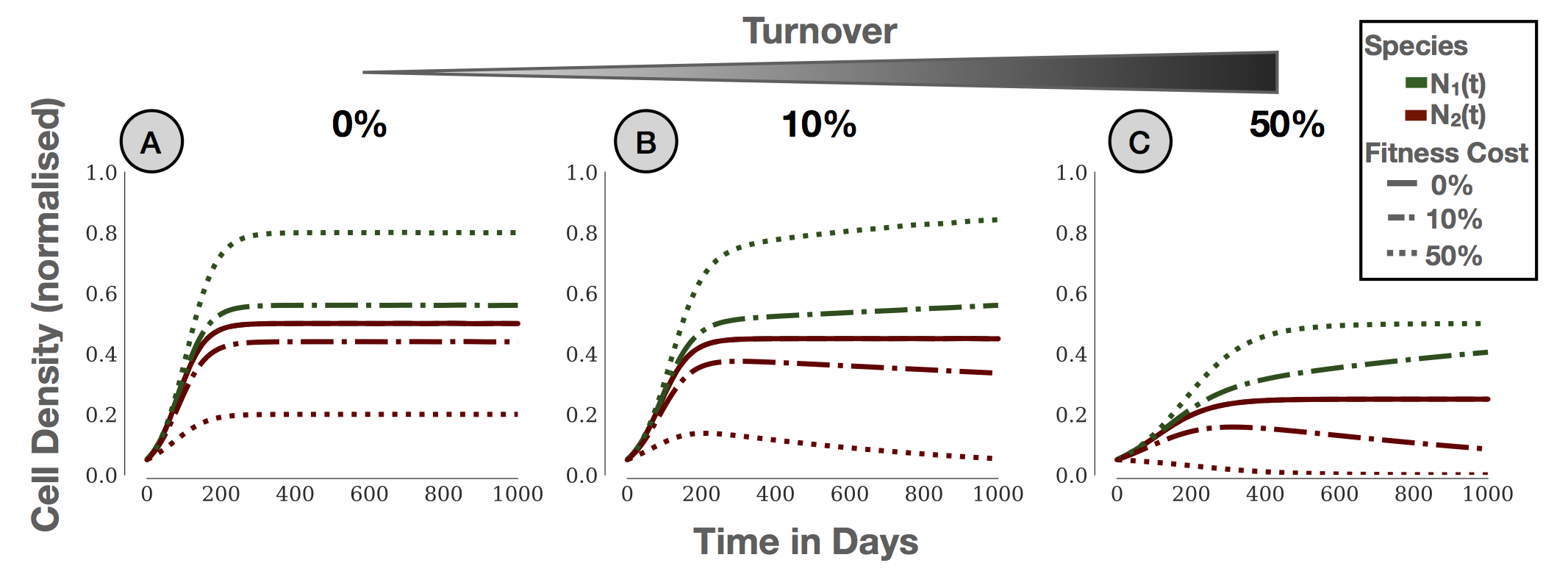

Figure 2: Interaction of two competing species modelled with the Lotka-Volterra model. Species 2 is assumed to have a reduced fitness. A) If we assume \(r\) and \(K\) are independent, the frequency of Species 2 decreases with its fitness, but Species 2 will never go extinct. This is because in assuming this independence, we are assuming that there is not turnover. B & C) When turnover is included, so that \(r\) and \(K\) are linked, the less fit species will go extinct over time. Parameters: \(r_1=0.027 d^{-1}, N_1(0) = N_2(0) = 0.05 K\). Reproduced from¹⁵.

Another, possibly even more important, reason for why the apparent independence of \(r\) and \(K\) in the \(r\)-\(K\) model is problematic, is seen when we use the logistic model to study the interaction between two species (say \(N_1\) and \(N_2\)). This yields the well-known Lotka-Volterra model: \begin{align*} \frac{d N_1(t)}{d t} &= r_1 \left(1-\frac{N_1+N_2}{K}\right) N_1 ,\\ \frac{d N_2(t)}{d t} &= r_2 \left(1-\frac{N_1+N_2}{K}\right) N_2. \end{align*} Say, Species 1 has growth rate \(r_1\) and is fitter than Species 2 which has growth rate \(r_2 < r_1\). Clearly, \(N_1\) should win over time, right? Interestingly, solving for the steady states of this system, the first thing we do is drop \(r_1\) and \(r_2\), so that they do not apparently influence the value of the final steady state - strange (see footnote 1)... What is going on?

\(r\) and \(K\) are not independent

The answer to this question lies in the definition of \(K\) - specifically, the fact that the \(r\)-\(K\) formulation makes it seem as if \(r\) and \(K\) are independent. To see why, let us return to the birth-death CA model. Writing out the birth and death process explicitly in the ODE model, we get the following equation: \begin{align*} \frac{d N(t)}{d t} &= \underbrace{\rho \left(1 - \frac{N}{K}\right) N}_{\text{Birth}} - \underbrace{\delta N}_{\text{Death}}, \\ &= \hat{r} \left(1 - \frac{N}{\hat{K}}\right) N, \end{align*} where \(\hat{r} = \rho - \delta\) and \(\hat{K} = \left(1-\frac{\delta}{\rho}\right)K\). Using this equation, we can now obtain the dependence of the long term equilibrium on \(\rho\) and \(\delta\) (see footnote 2). So, yes - we can write this equation in \(r\)-\(K\) form. However: \(K\) is dependent on \(r\). The population can never completely fill up the environment, because some cell somewhere will randomly die. By the time it's been replaced, another one will have died somewhere else - kind of like a game of wack-a-mole.

Explicitly adding the death term (or making the carrying capacity parameter of each population a function of its growth rate) also fixes the above inconsistency in the Lotka-Volterra model. If we assume non-zero death, the growth rates contribute to the steady states of this model, and the less fit population will go extinct over time (Figures 2B & C; for the maths see e.g. [8]). Finally, this also explains why it has been difficult to find evidence for for the \(r\)-\(K\) selection hypothesis - \(r\) and \(K\) are not independent (for more details see [8] and [4])!

What is a tumour's carrying capacity?

I stumbled upon the above discussion (in particular the excellent paper by Mallet⁸), whilst working on a model of adaptive therapy. There had been a lot of debate in the Anderson lab about the role of a fitness cost of resistance, and I thought I would use a simple Lotka-Volterra model to gain some intuition. Very quickly I ran into the problem I discussed above: the growth rates seemed to have less of an impact than I had expected. Moreover, while introducing a cost did increase the absolute time an adaptive therapy would gain compared to a continuous therapy, it did not change the relative time gained. Basically, if you didn't gain much without a cost you didn't gain much with a cost either (see our pre-print for more details). I couldn't quite pinpoint it at the time, but something bugged me about this result. It's not that I'm a strong believer in resistance costs - I think they are dependent on the environmental and genetic context - it was this ambivalence: if you don't benefit from adaptive therapy without a cost, you don't gain from a cost either.

Around that time, Fred Adler posted a blog post¹ on his concerns about the mathematical model used to motivate the adaptive therapy trial in prostate cancer. This post, and a comment left by Tom Bury led me to James Mallet's paper, and it clicked for me: what I had been missing was turnover! Without death, a fitness cost isn't really that big a deal - you just wait around for better times. Turnover changes this game: being slower at reproducing, either due to fitness costs, or due to competition, suddenly matter a lot more - your days are numbered. As such, both the impact of a fitness cost, and that of competition, depend on the cell turnover.

Tumours are a disease of up-regulated cell division. But how about cell death? How frequently does a tumour cell die - likely not very often, right? While we found it hard to find data on this topic (and if you have any recommendations, please post them below), to our surprise it seems like cell production and cell loss in tumours are closely balanced (e.g. [14]). On second thought, this actually makes sense: in homeostatic tissue cell birth and death is exactly balanced! This paints a rather dynamic picture of the tumour ecosystem - one in which cells are continuously replacing each other, and this rate will determine the speed of evolution towards, and away from resistance.

Conclusion

To sum up, we need to be careful with how exactly we interpret the parameters in the logistic growth model. Writing it in the \(r\)-\(K\) formulation is convenient, and makes it intuitive to fit data, which is why Raymond Pearl originally introduced it in the 1930s¹³. However, we have to remember that this \(K\) is dynamic. It is determined by space and resource availability, which will change as the tumour invades and recruits vasculature. In addition, it is also determined by the ratio of birth to death in the tumour. Specifically, if \(r\) changes, for example due to mutations or treatment, then so will \(K\). The amount by which it changes depends on the turnover. The shorter your life span, the more competition will matter. In the cancer world, this implies for example, that even a small fitness cost of resistance may have a much larger effect on the population than one might expect. This is the phenomenon we explore in our new pre-print¹⁵. In addition, if you would like to learn more about the mathematics of adaptive therapy I recommend Yannick Viossat’s and Rob Noble’s recent pre-print¹⁸. If this discussion intrigued you, head over to Biorxiv and check them out.

Finally, as a small disclaimer, I am not trying to advocate logistic growth as a tumour growth model. If you intend to quantitatively describe tumour growth, there is strong evidence that models such as the Gompertzian model are more suited (e.g. [10, 2]). And again the cancer world isn’t alone here: in 1920, Pearl and Reed used the logistic growth model to predict that the American population would saturate at 197 Million ¹³ - a fraction of what it is today. Instead, I think logistic growth provides a simple and intuitive model of population growth, which allows us to further our understanding of population biology and ecology - for example, the dependence between \(r\) and \(K\). Adopting the words of George Box: All models are wrong, but if used in the right context they are useful.

Footnotes

1. Technically speaking, the situation is a bit more complicated. In the above form of the Lotka-Volterra model, every point along the line \(N_1+N_2 = K\) is a steady state. Which point along this line a trajectory will converge to, depends on the ratio \(r_1/r_2\). However, unless we make this ratio infinite, Species 2 will never go extinct (Figure 2A) (jump back)

2. Interestingly the CA does not settle at \(\hat{K}\) but at \(\left(1-\frac{\delta}{\rho}\right)^{1/4}K\); see an upcoming pre-print by Gregory Kimmel et al. (jump back)

3. Thanks very much to Jeffrey West and Andrew Krause for many useful discussions, and helping me with this post. This wouldn’t have happened without you!

References

1. Frederick Adler. All pithy maxims about modeling are wrong, but some are useful - The Mathematical Oncology Blog.
2. Sebastien Benzekry, Clare Lamont, Afshin Beheshti, Amanda Tracz, John M.L. Ebos, Lynn Hlatky, and Philip Hahnfeldt. Classical Mathematical Models for Description and Prediction of Experimental Tumor Growth. PLoS Computational Biology, 10(8):e1003800, aug 2014.
3. Rafael R. Bravo, Etienne Baratchart, Jeffrey West, Ryan O. Schenck, Anna K. Miller, Jill Gallaher, Chandler D. Gatenbee, David Basanta, Mark Robertson-Tessi, and Alexander R. A. Anderson. Hybrid Automata Library: A flexible platform for hybrid modeling with real-time visualization. PLOS Computational Biology, 16(3):e1007635, mar 2020.
4. Jeremy Fox. Zombie ideas in ecology: r and k selection, 2011.
5. G. F. Gause and A. A. Witt. Behavior of Mixed Populations and the Problem of Natural Selection. The American Naturalist, 69(725):596–609, nov 1935.
6. Alfred J Lotka. Elements of physical biology. 1925.
7. Robert H MacArthur and Edward O Wilson. The theory of island biogeography, volume 1. Princeton university press, 2001.
8. James Mallet. The struggle for existence: how the notion of carrying capacity, K, obscures the links between demography, Darwinian evolution, and speciation. Evolutionary Ecology Research, 14(August):627–665, 2012.
9. T. R. Malthus. An Essay on the Principle of Population. Or a View of its Past and Present Effects on Human Happiness; with an Inquiry into our Prospects Respecting the Future Removal or Mitigation of the Evils which it Contains. John Murray, London, 1826.
10. M. Marusic, Bajzer, J. P. Freyer, and S. Vuk-Pavlovic. Analysis of growth of multicellular tumour spheroids by mathematical models. Cell Proliferation, 27(2):73–94, feb 1994.
11. AG McKendrick and M Kesava Pai. Xlv.—the rate of multiplication of micro-organisms: a mathematical study. Proceedings of the Royal Society of Edinburgh, 31:649–653, 1911.
12. Raymond Pearl. Introduction to medical biometry and statistics. WB Saunders, 1923.
13. Raymond Pearl and Lowell J Reed. On the rate of growth of the population of the united states since 1790 and its mathematical representation. Proceedings of the National Academy of Sciences of the United States of America, 6(6):275, 1920.
14. G G Steel. Cell loss as a factor in the growth rate of human tumours. European Journal of Cancer (1965), 3(4-5):381–387, 1967.
15. Maximilian Andreas Roland Strobl, Jeffrey West, Joel Brown, Robert Gatenby, Philip Maini, and Alexander Anderson. Turnover modulates the need for a cost of resistance in adaptive therapy. BioRxiv, 2020.
16. Pierre-Francois Verhulst. Notice sur la loi que la population suit dans son accroissement. Corresp. Math. Phys., 10:113–126, 1838.
17. Yannick Viossat and Robert John Noble. The logic of containing tumors. bioRxiv, page 2020.01.22.915355, jan 2020.
18. Wikipedia. r/k selection, 2020.