---

Introduction:

The primary job of a mathematical modeler is to create equations that are an accurate representation of the biological system under investigation. Often this is accomplished by combining intuition, experience, existing model forms, and iteration to arrive at a reasonable model that is both mathematically appropriate and physiologically realistic. But what if there was a data-informed way to identify a model’s key terms?

Equation learning is a recent area of research to develop methods that directly learn unknown model dynamics from data. There are many different ways to learn equations, but a common approach trains neural networks (NNs) to approximate the solutions of a differential equation model and/or the unknown dynamics in the model.

There are several variations to this general mechanistic machine learning approach. We review three methods below, each imposing additional constraints and with various levels of pre-existing knowledge built into the form of the equation. In general, this mechanistic machine learning approach is exciting because it allows the modeler to maintain a high degree of flexibility when the mechanisms underlying the system are not well known and learn the model behavior and structure from available data. However, while the approach appears quite promising, most research to date has only applied these techniques to high-resolution in silico data where the underlying ground truth is known. In the biological context, data are often sparse and noisy, which challenges the applications of these methods. In this blog post we briefly review three methods to learn dynamics from data that handle noisy and sparse data differently, and speculate how mathematical oncology can benefit from these approaches.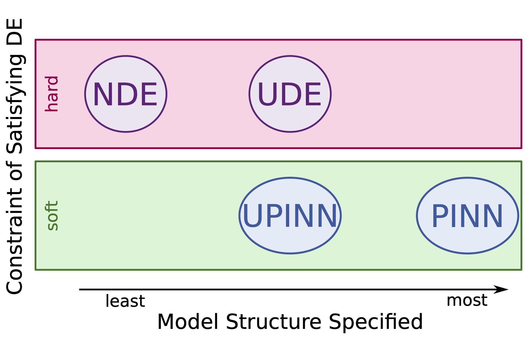

Learning Unknown Dynamics:

The methods that use NNs to parametrize or learn unknown dynamics in differential equation models can be classified in several ways. Firstly, by how specified the differential equation (DE) model structure is (including the number of known terms, if any), and secondly, how strictly the DE model is enforced during NN training. See Figure 1 for a mapping of several methods with respect to these classifiers. The most rigid method (in terms of specifying the model structure) is called physics informed neural networks (PINNs), which assume the model structure is completely known [1]. The most flexible method along this axis is called a neural differential equation (NDE), which assumes no known structure at all and learns the entire model dynamics with a NN. In between these two extreme cases are two methods that have partially defined model structure and partially unknown structure. These two methods, called universal differential equations (UDEs) [2] and universal physics informed neural networks (UPINNs), use a NN to learn the partially unknown model structure [3,4,5].

Regarding how strictly the DE model is enforced during NN training, NDEs and UDEs are trained to exactly solve the learned DE models; this is referred to as a “hard constraint.” UPINNs and PINNs, on the other hand, are only trained to approximately solve their learned DEs, which is referred to as a “soft constraint”. Figure 1 maps the four methods in terms of their constraints and specified model structures. Note that PINNs cannot learn new dynamics while the other three methods can, so we do not consider it as an equation learning method in this blog. Below we describe the three equation-learning methods in more detail. For simplicity, we focus on explicit first order differential equations given by , $$ \begin{equation} \frac{dx}{dt}=f(x,t) \end{equation} $$ however, the differential equations used in these methods may be more general ordinary or partial differential equations, depending on the modeling context.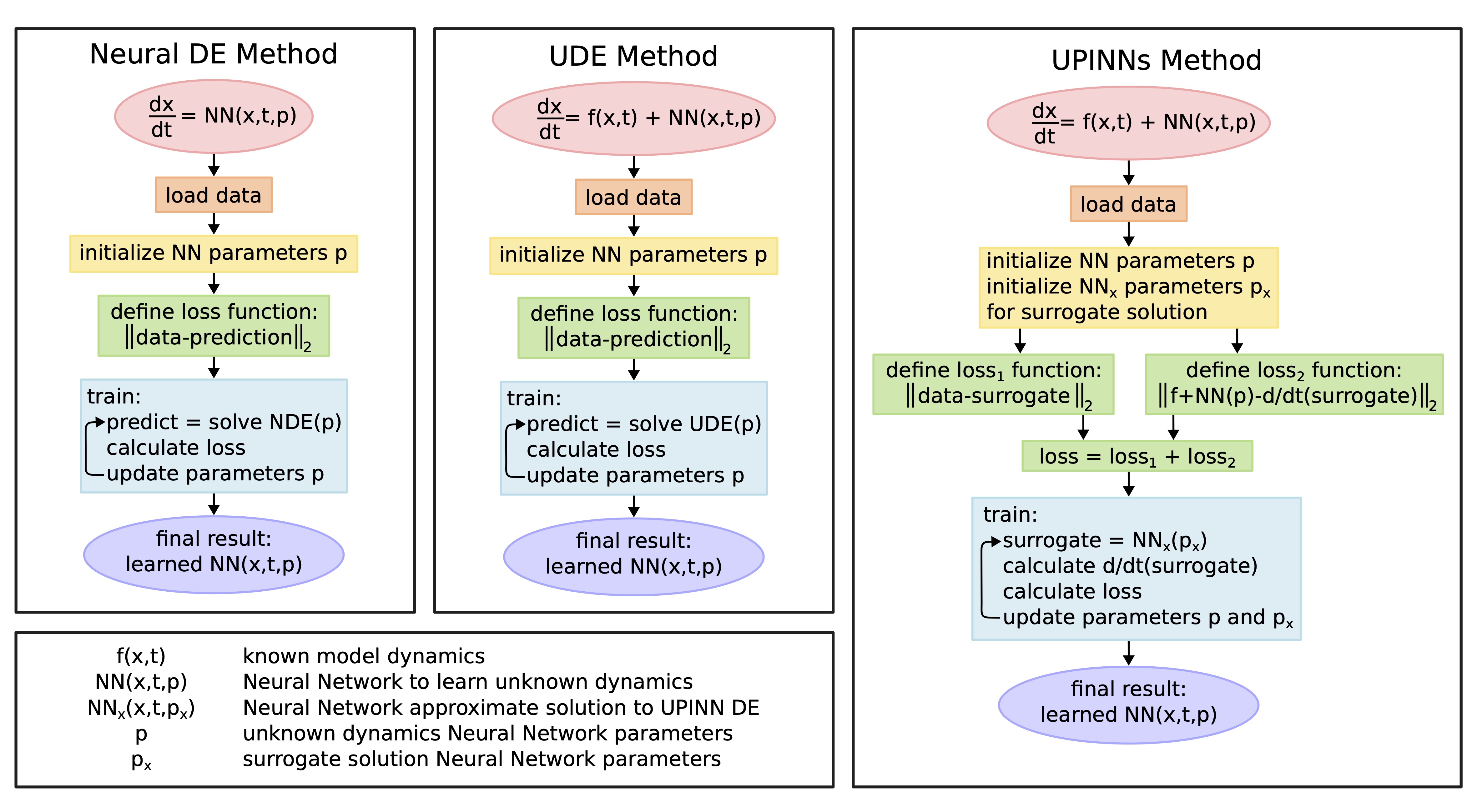

Of course, as mathematical modelers, we often seek to have closed-form expressions for the right hand side of a differential equation. With each of these approaches, a second step can be used to determine the model terms, usually using symbolic regression. Two popular methods are SINDy (Sparse Identification of Nonlinear Dynamics) and AI Feynman [6,7], but there are many more. SINDy requires the user to provide a library of candidate functions (e.g., polynomials) and employs regularization, such as LASSO, to select the most parsimonious model. In contrast, AI Feynman exploits properties of physical equations (e.g., symmetry, polynomials, compositionality) along with NNs to perform symbolic regression.

Neural Differential Equation (Neural DE):

The most flexible method that combines NNs and differential equations is called a Neural Differential Equation, or Neural DE (NDE). This method replaces the entire right-hand-side of a differential equation with a NN. It assumes no prior knowledge in model structure and is fully informed by the available data. The NN on the right-hand side of the DE depends on the state of the system, x(t), time, t, and many NN parameters, p (a set of weights and biases in the case of multilayer perceptron networks). The NN is trained to minimize a loss function, typically the error between the numerical solution of the NDE and the data. As the differential equation always holds, it is a hard constraint.

This method provides a great deal of flexibility and generality since it does not require prior knowledge of model structure. This flexibility comes with a trade-off, however, as the NN - a universal function approximator - with high complexity and number of parameters, leads to the risk of overfitting and is highly sensitive to noise in the data.

Universal Differential Equation (UDE):

Universal Differential Equations (UDEs) are an extension of NDEs. Specifically, UDEs allow the modeler to incorporate known terms into the right hand side of the differential equation. Thus, the form of a UDE’s right-hand-side consists of known model terms (e.g., logistic growth) and one NN that represents the remaining unknown model structure. The NN is trained in the same manner as the NDE described above and thus also enforce the DE as a hard constraint. The advantage to such an approach is that it incorporates prior knowledge into the dynamic-learning problem through the addition of partially-known model structure, reducing the sensitivity of the method to limited or noisy data compared to the NDE case.

Universal Physics-Informed Neural Network (UPINN):

We begin with a short description of physics-informed neural networks (PINNs) before discussing Universal PINNs (UPINNs). PINNs are the most rigid approach, in that the model structure is entirely prescribed, and only parameter values are unknown and learned from data. Here, a NN is used as a surrogate for the solution to the DE model as an alternative to solving the DE with numeric integration. This NN is trained simultaneously to fit a given dataset, if available, and satisfy the prescribed DE model - making the DE a soft constraint. Unknown parameter values can be estimated during the training process as well. An advantage of this approach over normal curve-fitting methods is that it performs well with sparse and noisy datasets. The original PINNs study demonstrated that the solution to Schrodinger’s equation could be predicted over the entire spatio-temporal domain using just data from the initial condition and boundaries [1]. Datasets from oncology are often noisy and sparse. PINNS-based approaches may be a valuable addition to mathematical oncology techniques because they are more robust to these traditionally quite challenging data limitations.

Universal PINNs (UPINNs) are an extension of the PINNs approach where one uses two NNs: one as a surrogate to the solution of the DE, and another for the unknown terms in the right-hand-side of the DE. In doing so, this approach leverages advantages of both the PINNs and UDEs approaches. Similar to a PINN, this approach is robust to noisy and sparse data. Similar to a UDE, it can learn unknown dynamics from data. The training process of UPINNs is similar to that of PINNs. All NNs are simultaneously trained to minimize a total loss function, which is the sum of two loss functions: one to ensure the surrogate solution closely matches the data, and a second to ensure the NNs approximately satisfy the prescribed DE model (with known and unknown dynamics and as a soft constraint). In the total loss function there is an important trade-off between satisfying the data and satisfying the DE. Compared to the UDE/NDE approach, the UPINN approach is more robust to sparse and/or noisy data because it isn’t required to satisfy the DE as a hard constraint. Podina and colleagues demonstrated in a specific example that the UPINN method is more robust to noise and data sparsity when learning unknown model dynamics than the UDE approach [8].

Conclusion

The advantages and differences of these dynamic-learning methods are clearly evident in the table above: a framework that balances the ability to programmatically find new, non-intuitive model dynamics that fit the data while at the same time allowing the modeler to insert prior knowledge and build desired constraints into the model structure.

While there is potential for biological and clinical applications, neural network-based methods like these can be prone to overfitting, learning overly complex dynamics and consequently identifying extra model terms that overfit the data’s inherent noise. PINNs-based approaches try to moderate this weakness by changing the differential equation to a soft constraint – allowing some leniency in the resulting solution that can moderate the effects of noise and sparse data. Traditional modeling approaches do not extensively explore a range of model structures and are limited by the modeler’s choices and biases, as they draw from the proverbial hat of known modeling forms. To account for our own biases and aid with model selection and data-informed model building, these new equation-learning methods certainly have a role to play in future mathematical oncology applications. Already the first applications have been successful in learning cellular behaviours from in vitro experiments [9]. The next step would be to incorporate these newly learned behaviours into in vivo models with matching data. Certainly, the future of mathematical oncology is exciting, as new methods, like the ones discussed here, lead to newly discovered dynamics, new modeling tools, and improved understanding of cancer and its treatment.

References

1. Raissi, M., Perdikaris, P. and Karniadakis, G.E., 2019. Physics-informed neural networks: A deep learning framework for solving forward and inverse problems involving nonlinear partial differential equations. Journal of Computational physics, 378, pp.686-707.
2. Rackauckas, C., Ma, Y., Martensen, J., Warner, C., Zubov, K., Supekar, R., Skinner, D., Ramadhan, A. and Edelman, A., 2020. Universal differential equations for scientific machine learning. arXiv preprint arXiv:2001.04385.
3. Chen, Z., Liu, Y. and Sun, H., 2021. Physics-informed learning of governing equations from scarce data. Nature communications, 12(1), p.6136.
4. Pang, G. and Karniadakis, G.E., 2020. Physics-informed learning machines for partial differential equations: Gaussian processes versus neural networks. Emerging frontiers in nonlinear science, pp.323-343.
5. Grossmann, T.G., Komorowska, U.J., Latz, J. and Schönlieb, C.B., 2024. Can physics-informed neural networks beat the finite element method?. IMA Journal of Applied Mathematics, p.hxae011.
6. Udrescu, S.M. and Tegmark, M., 2020. AI Feynman: A physics-inspired method for symbolic regression. Science advances, 6(16), p.eaay2631.
7. Brunton, S.L., Proctor, J.L. and Kutz, J.N., 2016. Discovering governing equations from data by sparse identification of nonlinear dynamical systems. Proceedings of the national academy of sciences, 113(15), pp.3932-3937.
8. Podina, L., Eastman, B. and Kohandel, M., 2023, July. Universal physics-informed neural networks: symbolic differential operator discovery with sparse data. In International conference on machine learning (pp. 27948-27956). PMLR.
9. Podina, L., Ghodsi, A. and Kohandel, M., 2024. Learning chemotherapy drug action via universal physics-informed neural networks. arXiv preprint arXiv:2404.08019.